Step-by-Step in Databricks: Creating a Date and Time dimension for BI Analytics

In this article, you will learn how to set up date and time dimensions in Databricks to enable precise time-based analyses and reports.

Intro

In the world of business intelligence (BI), data structures that enable clear, consistent analysis are of central importance. Two fundamental concepts in this context are dimensions and facts. But what is behind these terms?

Facts represent the quantitative data that is collected and analyzed in a company. They answer questions such as “How many sales were made?”, “What is the turnover?” or “How many hours were worked?” These facts provide the real value of BI analysis, as they show measurable results and performance.

Dimensions, on the other hand, are qualitative data that serve as a context for the analysis. They help to organize facts into meaningful groups. A dimension describes a specific perspective from which the facts can be viewed - for example, customer data, products, geographical regions, or even time. Dimensions make it possible to structure analyses according to relevant characteristics and answer questions such as “When were the most sales made?” or “Which products are particularly popular in a particular quarter?”.

Within the dimensions, the Date and Time dimensions occupy a prominent position. As time is a universal constant in the business world, it forms the basis for comparisons, developments, and predictions.

Dimension Date

The Date dimension is the structure that encompasses the entire calendar system. It makes it possible to organize and analyze data across different time periods. Typically, a date dimension contains attributes such as year, quarter, month, and day, as well as specific calendar events such as holidays, fiscal year periods, and seasonal labels. The date dimension is essential for carrying out analyses over longer periods of time and recognizing long-term trends. For example, it enables companies to examine turnover on a quarterly basis, analyze seasonal sales figures, or determine the impact of public holidays on demand.

Dimension Time

The Time dimension goes one level deeper and refers to the breakdown of the calendar day into smaller units such as hours, minutes, and seconds. This dimension is particularly important in use cases where time plays a role within a day - e.g., when analyzing response times in a call center, when looking at production processes in manufacturing, or when analyzing user activities on a website. The time dimension enables detailed insights into time periods that extend beyond the daily boundary and thus helps to identify patterns that are influenced by intra-day fluctuations.

Where are the dimensions created?

Date and time dimensions are typically created in the data warehouse or lakehouse - i.e., directly in a platform such as Databricks.

Here are a few reasons why you should not create the date and time dimensions in a visualization tool such as Power BI or Tableau:

Central data source
If the date and time dimensions are created in the data warehouse or lakehouse, they are available centrally to all data applications and tools. This prevents different teams from creating or using different time dimensions, which ensures the consistency of the data and analyses.
Efficiency and performance
Time dimensions are often large tables, as they have to cover a large number of points in time and dates. Storing and querying such tables is much more efficient in the DWH/Lakehouse than in a BI tool, as these platforms are designed for large amounts of data.
Transformation and flexibility
In a system like Databricks, date, and time dimensions can be easily customized and extended to cover specific requirements, such as custom calendars, holidays, or fiscal periods. These transformation options would be limited and often more cumbersome in a BI tool like Power BI.
Reusability
The created date and time dimensions can then be easily integrated into the BI tool. Power BI or another tool accesses the prepared dimension tables so that no additional transformations or manual work is necessary.

In practice, you create the date and time dimensions in Databricks (or a similar lakehouse/DWH system) and then use them in Power BI for visualizations and reports.

Below, I explain how to create such dimensions.

Get started for free with Databricks

Databricks recently started offering the opportunity to test a managed account directly at Databricks itself and receive a starting credit of 400 US dollars. Databricks manages the entire cloud structure. A great thing is that within a few minutes, you are ready to go. You can access the trial on the following page:

https://login.databricks.com/

There is a choice between Professional Use and Personal Use. Personal Use is the Community Edition of Databricks, which is now a little outdated and does not offer the same functionalities.

With Express Setup, you are ready to go in no time at all.

The code

After the theory, I will now put the concepts into practice. To do this, I will create a new notebook in Databricks. I already have a catalog “demo” in which I want to deploy the tables and views, which I will create in the schema “silver”.

For data manipulation and transformation tasks in PySpark, I need some PySpark Libraries. So I will import them in the first step.

1
2
3


from pyspark.sql.types import LongType

from pyspark.sql.functions import year, month, day, hour, minute, second, col, expr, when, date_format, lit, to_timestamp, min, max, ceil, to_date

So that the notebook can be kept generic, I will create three widgets in which the catalog can be specified, as well as the start and end date. This means that the corresponding date dimension will be created exactly in this period. I have a large period from January 1, 1990 to December 31, 2050.

1
2
3


dbutils.widgets.text('start_date',  '1990-01-01',   'Start Date')
dbutils.widgets.text('end_date',    '2050-12-31',   'End Date')
dbutils.widgets.text('catalog',     'demo',         'Catalog')

Then I pack the input of the widgets into variables, I also create variables for the table names and print them out.

 1
 2
 3
 4
 5
 6
 7
 8
 9
10
11
12
13


start_date            = dbutils.widgets.get('start_date')
end_date              = dbutils.widgets.get('end_date')
catalog               = dbutils.widgets.get('catalog')
date_table            = f'{catalog}.silver.dim_date'
time_minute_table     = f'{catalog}.silver.dim_time_minute'
mapping_minute_table  = f'{catalog}.silver.dim_mapping_minute'

print(f'Create Dimension Tables for Date and Time')
print(f'Timerange: {start_date} to {end_date}')
print(f'Create the following tables: ')
print(f'{date_table}')
print(f'{time_minute_table}')
print(f'{mapping_minute_table}')

If the Silver and Gold scheme does not yet exist, I will create it.

1
2


spark.sql(f"CREATE SCHEMA IF NOT EXISTS {catalog}.silver").display()
spark.sql(f"CREATE SCHEMA IF NOT EXISTS {catalog}.gold").display()

So that I can use translations later, I will install various dictionaries in which I will enter the translations.

Below is the explanation for the translation dictionaries.

months_dict: Maps English month names to their translations and abbreviations in German, French, and Italian.

days_dict: Maps English day names to their translations and abbreviations in German, French, and Italian.

date_mapping_dict: Combines months_dict and days_dict into a single dictionary for easier access.

 1
 2
 3
 4
 5
 6
 7
 8
 9
10
11
12
13
14
15
16
17
18
19
20
21
22
23
24
25
26
27
28


# Translation and abbreviated translation for German, French, and Italian 
months_dict = {
    "January":    ["Januar",    "Jan.", "janvier",     "janv.", "gennaio",    "gen."],
    "February":   ["Februar",   "Feb.", "février",     "fév.",  "febbraio",   "feb."],
    "March":      ["März",      "Mär.", "mars",        "mar.",  "marzo",      "mar."],
    "April":      ["April",     "Apr.", "avril",       "avr.",  "aprile",     "apr."],
    "May":        ["Mai",       "Mai.", "mai",         "mai.",  "maggio",     "mag."],
    "June":       ["Juni",      "Jun.", "juin",        "jui.",  "giugno",     "giu."],
    "July":       ["Juli",      "Jul.", "juillet",     "juil.", "luglio",     "lug."],
    "August":     ["August",    "Aug.", "août",        "aoû.",  "agosto",     "ago."],
    "September":  ["September", "Sep.", "septembre",   "sept.", "settembre",  "set."],
    "October":    ["Oktober",   "Okt.", "octobre",     "oct.",  "ottobre",    "ott."],
    "November":   ["November",  "Nov.", "novembre",    "nov.",  "novembre",   "nov."],
    "December":   ["Dezember",  "Dez.", "décembre",    "déc.",  "dicembre",   "dic."],
}

# Translation and abbreviated translation for German, French, and Italian
days_dict = {
    "Monday":     ["Montag",      "Mo.", "lundi",    "lun.", "lunedì",    "lun."],
    "Tuesday":    ["Dienstag",    "Di.", "mardi",    "mar.", "martedì",   "mar."],
    "Wednesday":  ["Mittwoch",    "Mi.", "mercredi", "mer.", "mercoledì", "mer."],
    "Thursday":   ["Donnerstag",  "Do.", "jeudi",    "jeu.", "giovedì",   "gio."],
    "Friday":     ["Freitag",     "Fr.", "vendredi", "ven.", "venerdì",   "ven."],
    "Saturday":   ["Samstag",     "Sa.", "samedi",   "sam.", "sabato",    "sab."],
    "Sunday":     ["Sonntag",     "So.", "dimanche", "dim.", "domenica",  "dom."],
}

date_mapping_dict = {"Months": months_dict, "Days": days_dict}

I will also create a dictionary so that I can map time intervals.

time_mapping_dict: Defines mappings for different time window groups (e.g., 5-minute, 10-minute intervals) to their respective ranges within an hour. Each key (e.g., “5Min”, “10Min”) represents a time window group, and the values are dictionaries that map an interval number to a time range string.

 1
 2
 3
 4
 5
 6
 7
 8
 9
10
11
12
13
14
15
16
17
18
19
20
21
22
23
24
25
26
27
28
29
30
31
32
33
34
35
36
37
38
39
40
41
42
43


# Define the nested mapping dictionary for different window groups
time_mapping_dict = {
    "5Min": {
        1: "00-05",
        2: "05-10",
        3: "10-15",
        4: "15-20",
        5: "20-25",
        6: "25-30",
        7: "30-35",
        8: "35-40",
        9: "40-45",
        10: "45-50",
        11: "50-55",
        12: "55-60"
    },
    "10Min": {
        1: "00-10",
        2: "10-20",
        3: "20-30",
        4: "30-40",
        5: "40-50",
        6: "50-60"
    },
    "15Min": {
        1: "00-15",
        2: "15-30",
        3: "30-45",
        4: "45-60"
    },
    "20Min": {
        1: "00-20",
        2: "20-40",
        3: "40-60"
    },
    "30Min": {
        1: "00-30",
        2: "30-60"
    },
    "60Min": {
        1: "00-60"
    }
}

So that I can map the time values to the corresponding window group, I create a corresponding user-defined function (UDF).

 1
 2
 3
 4
 5
 6
 7
 8
 9
10
11
12
13


# Create a UDF to map the time values to the corresponding window group
get_window_group = udf(
    lambda minute, window_type: time_mapping_dict[window_type][
        next(
            (
                group
                for group, window in time_mapping_dict[window_type].items()
                if int(window.split("-")[0]) <= minute < int(window.split("-")[1])
            ),
            0,
        )
    ]
)

So that I can create the Time Windows, I have written the following function.

 1
 2
 3
 4
 5
 6
 7
 8
 9
10
11
12
13
14
15
16
17
18
19
20
21
22
23
24
25
26
27
28


def create_time_window(df, duration, timestampCol="TimestampStartUtc", minuteCol="TimeMinute", secondCol="TimeSecond"):
  """
  Adds time window columns to the given dataframe.

  Parameters:
  df (DataFrame): Input dataframe.
  duration (int): Duration of the time window in minutes.
  timestampCol (str): Column name for the timestamp. Default is "TimestampStartUtc".
  minuteCol (str): Column name for the minute. Default is "TimeMinute".
  secondCol (str): Column name for the second. Default is "TimeSecond".

  Returns:
  DataFrame: Dataframe with added columns:
    - IsWindow<duration>MinuteStart: Boolean indicating if the minute is the start of a window.
    - Window<duration>MinuteId: Integer ID of the window group.
    - Window<duration>MinuteName: String name of the window group.
  """
  
  is_window_start = f"IsWindow{duration}MinuteStart"
  window_id = f"Window{duration}MinuteId"
  window_name = f"Window{duration}MinuteName"
    
  df = (df
        .withColumn(is_window_start, when((col(minuteCol) % duration == 0) & (col(secondCol) == 0), True).otherwise(False))
        .withColumn(window_id, ceil((col(minuteCol) + 1) / duration).cast("integer"))
        .withColumn(window_name, get_window_group(minuteCol, lit(f"{duration}Min")))
      )
  return df

In the next step, I will create a function that adds additional columns to the date dataframe. How wide or how many columns can this table have? From my point of view, the more the better 😊. As the table is in Silver, a view can be placed on it in Gold, in which you can then only select the columns that will be used in the report.

  1
  2
  3
  4
  5
  6
  7
  8
  9
 10
 11
 12
 13
 14
 15
 16
 17
 18
 19
 20
 21
 22
 23
 24
 25
 26
 27
 28
 29
 30
 31
 32
 33
 34
 35
 36
 37
 38
 39
 40
 41
 42
 43
 44
 45
 46
 47
 48
 49
 50
 51
 52
 53
 54
 55
 56
 57
 58
 59
 60
 61
 62
 63
 64
 65
 66
 67
 68
 69
 70
 71
 72
 73
 74
 75
 76
 77
 78
 79
 80
 81
 82
 83
 84
 85
 86
 87
 88
 89
 90
 91
 92
 93
 94
 95
 96
 97
 98
 99
100
101
102
103
104
105
106
107
108
109
110
111
112
113
114
115
116
117
118
119
120
121
122
123
124
125
126
127
128
129
130
131
132
133
134
135
136
137
138
139
140


def add_date_columns(df):
  """
  Function to add date-related columns.
  
  Parameters:
  df (DataFrame): Input dataframe with a 'Date' column.
  
  Returns:
  DataFrame: Dataframe with added date-related columns.
  List[str]: List of the added date-related column names.

  The added columns include:
    - DatePK: Primary key for the date in the format YYYYMMDD.
    - DateString: Date formatted as dd.MM.yyyy.
    - Year: Year of the date.
    - IsLeapYear: Boolean indicating if the year is a leap year.
    - HalfYearId: Half of the year (1 for Jan-Jun, 2 for Jul-Dec).
    - YearHalfYearId: Unique identifier for the half-year.
    - HalfYearName: Name of the half-year (H1 or H2).
    - YearHalfYear: Combination of year and half-year name.
    - Quarter: Quarter of the year (1 to 4).
    - YearQuarterId: Unique identifier for the quarter.
    - YearQuarter: Combination of year and quarter.
    - QuarterShortname: Short name for the quarter (Q1 to Q4).
    - YearMonthId: Unique identifier for the year and month.
    - Month: Month of the date.
    - MonthName: Full name of the month.
    - MonthNameShort: Short name of the month.
    - MonthNameDe: Full name of the month in German.
    - MonthNameShortDe: Short name of the month in German.
    - MonthNameFr: Full name of the month in French.
    - MonthNameShortFr: Short name of the month in French.
    - MonthNameIt: Full name of the month in Italian.
    - MonthNameShortIt: Short name of the month in Italian.
    - WeekIdIso: ISO week number of the year.
    - WeekOfYearIso: ISO week number.
    - WeekOfYearIsoName: ISO week number with 'W' prefix.
    - YearWeekOfYearIso: Combination of year and ISO week number.
    - DayName: Full name of the day.
    - DayNameShort: Short name of the day.
    - DayNameDe: Full name of the day in German.
    - DayNameShortDe: Short name of the day in German.
    - DayNameFr: Full name of the day in French.
    - DayNameShortFr: Short name of the day in French.
    - DayNameIt: Full name of the day in Italian.
    - DayNameShortIt: Short name of the day in Italian.
    - DayOfYear: Day of the year.
    - Day: Day of the month.
    - DayOfWeekUs: Day of the week (0=Sunday, 6=Saturday).
    - DayOfWeekIso: ISO day of the week (1=Monday, 7=Sunday).
    - IsWeekDay: Boolean indicating if the day is a weekday.
    - IsLastDayOfMonth: Boolean indicating if the day is the last day of the month.
    - LastDayOfMonth: Last day of the month.
    - MonthDay: Date with the same day and month but year 1972.
    - StartOfWeekUs: Start date of the week (US).
    - StartOfWeekIso: Start date of the week (ISO).
    - EndOfWeekUs: End date of the week (US).
    - EndOfWeekIso: End date of the week (ISO).
    - IsHoliday: Boolean indicating if the day is a holiday.
  """
  #date
  df = (df
        .withColumn("DatePK", expr("year(Date) * 10000 + month(Date) * 100 + day(Date)"))
        .withColumn("DateString", expr("date_format(Date, 'dd.MM.yyyy')"))
      )

  #year
  df = (df
        .withColumn("Year", year(col("Date")))
        .withColumn("IsLeapYear",when((expr("year(Date) % 4 == 0") & expr("year(Date) % 100 != 0")) | expr("year(Date) % 400 == 0"), True).otherwise(False))
        # How to calculate leap year: https://learn.microsoft.com/en-us/office/troubleshoot/excel/determine-a-leap-year
      )

  #halfyear
  df = (df
        .withColumn("HalfYearId",when(month(df["Date"]).between(1, 6), 1).otherwise(2))
        .withColumn("YearHalfYearId",col("Year")*10+col("HalfYearId"))
        .withColumn("HalfYearName",when(month(df["Date"]).between(1, 6), "H1").otherwise("H2"))
        .withColumn("YearHalfYear", expr("concat(Year,'-', HalfYearName)"))
      )

  #quarter
  df = (df
        .withColumn("Quarter", expr("quarter(Date)")) 
        .withColumn("YearQuarterId", expr("year(Date) * 10 + quarter(Date)"))
        .withColumn("YearQuarter", expr("concat(Year,'-Q', quarter(Date))"))
        .withColumn("QuarterShortname", expr("concat('Q', quarter(Date))"))
      )

  #month
  df = (df
        .withColumn("YearMonthId", expr("CAST(date_format(Date, 'yyyyMM') AS INT)"))
        .withColumn("Month", month("Date"))
        .withColumn("MonthName", expr("date_format(Date, 'MMMM')"))
        .withColumn("MonthNameShort", expr("date_format(Date, 'MMM')"))
        .withColumn("MonthNameDe",expr("CASE "+ " ".join(["WHEN MonthName == '{0}' THEN '{1}'".format(k, v[0])for k, v in date_mapping_dict["Months"].items()])+ " END"),)
        .withColumn("MonthNameShortDe",expr("CASE "+ " ".join(["WHEN MonthName == '{0}' THEN '{1}'".format(k, v[1])for k, v in date_mapping_dict["Months"].items()])+ " END"),)
        .withColumn("MonthNameFr",expr("CASE "+ " ".join(["WHEN MonthName == '{0}' THEN '{1}'".format(k, v[2])for k, v in date_mapping_dict["Months"].items()])+ " END"),)
        .withColumn("MonthNameShortFr",expr("CASE "+ " ".join(["WHEN MonthName == '{0}' THEN '{1}'".format(k, v[3])for k, v in date_mapping_dict["Months"].items()])+ " END"),)
        .withColumn("MonthNameIt",expr("CASE "+ " ".join(["WHEN MonthName == '{0}' THEN '{1}'".format(k, v[4])for k, v in date_mapping_dict["Months"].items()])+ " END"),)
        .withColumn("MonthNameShortIt",expr("CASE "+ " ".join(["WHEN MonthName == '{0}' THEN '{1}'".format(k, v[5])for k, v in date_mapping_dict["Months"].items()])+ " END"),)
      )

  #week
  df = (df
        .withColumn("WeekIdIso", expr("year(Date) * 100 + extract(WEEKS FROM Date)"))
        .withColumn("WeekOfYearIso", expr("extract(WEEKS FROM Date)"))
        .withColumn("WeekOfYearIsoName", expr("concat('W', WeekOfYearIso)"))
        # the number of the ISO 8601 week-of-week-based-year. A week is considered to start on a Monday and week 1 is the first week with >3 days. In the ISO week-numbering system, it is possible for early-January dates to be part of the 52nd or 53rd week of the previous year, and for late-December dates to be part of the first week of the next year. For example, 2005-01-02 is part of the 53rd week of year 2004,  while 2012-12-31 is part of the first week of 2013.
        .withColumn("YearWeekOfYearIso", expr("concat(Year,'-', WeekOfYearIsoName)"))
      )

  #day
  df = (df
        .withColumn("DayName", expr("date_format(Date, 'EEEE')"))
        .withColumn("DayNameShort", expr("date_format(Date, 'EEE')"))
        .withColumn("DayNameDe",expr("CASE "+ " ".join(["WHEN DayName == '{0}' THEN '{1}'".format(k, v[0])for k, v in date_mapping_dict["Days"].items()])+ " END"),)
        .withColumn("DayNameShortDe",expr("CASE "+ " ".join(["WHEN DayName == '{0}' THEN '{1}'".format(k, v[1])for k, v in date_mapping_dict["Days"].items()])+ " END"),)
        .withColumn("DayNameFr",expr("CASE "+ " ".join(["WHEN DayName == '{0}' THEN '{1}'".format(k, v[2])for k, v in date_mapping_dict["Days"].items()])+ " END"),)
        .withColumn("DayNameShortFr",expr("CASE "+ " ".join(["WHEN DayName == '{0}' THEN '{1}'".format(k, v[3])for k, v in date_mapping_dict["Days"].items()])+ " END"),)
        .withColumn("DayNameIt",expr("CASE "+ " ".join(["WHEN DayName == '{0}' THEN '{1}'".format(k, v[4])for k, v in date_mapping_dict["Days"].items()])+ " END"),)
        .withColumn("DayNameShortIt",expr("CASE "+ " ".join(["WHEN DayName == '{0}' THEN '{1}'".format(k, v[5])for k, v in date_mapping_dict["Days"].items()])+ " END"),)
        .withColumn("DayOfYear", expr("dayofyear(Date)"))
        .withColumn("Day", expr("dayofmonth(Date)"))
        .withColumn("DayOfWeekUs", expr("extract(DOW FROM Date)"))
        .withColumn("DayOfWeekIso", expr("extract(DOW_ISO FROM Date)"))
        .withColumn("IsWeekDay", expr("DayOfWeekIso < 6"))
        .withColumn("IsLastDayOfMonth", expr("Date = last_day(Date)"))
        .withColumn("LastDayOfMonth", expr("last_day(Date)"))
        .withColumn("MonthDay", expr("make_date(1972, Month, Day)"))
        .withColumn("StartOfWeekUs", expr("date_sub(Date, DayOfWeekUs-1)"))
        .withColumn("StartOfWeekIso", expr("date_sub(Date, DayOfWeekIso-1)"))
        .withColumn("EndOfWeekUs", expr("date_add(Date, 7-DayOfWeekUs)"))
        .withColumn("EndOfWeekIso", expr("date_add(Date, 7-DayOfWeekIso)"))
        .withColumn("IsHoliday", lit(None).cast("boolean"))
      )
  
  date_columns = df.columns

  return df, date_columns

I have also created a function for the time dimension that adds additional columns and information.

 1
 2
 3
 4
 5
 6
 7
 8
 9
10
11
12
13
14
15
16
17
18
19
20
21
22
23
24
25
26
27
28
29
30
31
32
33
34
35
36
37
38
39
40
41
42
43
44
45
46
47
48
49
50
51
52
53
54
55
56


def add_time_columns(df):
  """
  Adds time-related columns to the given dataframe.

  Parameters:
  df (DataFrame): Input dataframe with a 'TimestampPK' column representing seconds since epoch.

  Returns:
  DataFrame: Dataframe with added time-related columns.
  List[str]: List of the added time-related column names.
  
  The added columns include:
    - TimestampStartUtc: Timestamp in UTC.
    - TimePK: Time in seconds since the start of the day.
    - Time: Time as a timestamp.
    - TimeString: Time formatted as HH:mm:ss.
    - TimeHour: Hour of the time.
    - TimeMinute: Minute of the time.
    - TimeSecond: Second of the time.
    - AmPm: AM/PM indicator.
    - TimeSecondId: Unique identifier for each second of the day.
    - TimeMinuteId: Unique identifier for each minute of the day.
    - IsWindow<duration>MinuteStart: Boolean indicating if the minute is the start of a window.
    - Window<duration>MinuteId: Integer ID of the window group.
    - Window<duration>MinuteName: String name of the window group.
  """
  # generate timestamps from TimePK
  df = (df
        .withColumn("TimestampStartUtc", col("TimestampPK").cast("timestamp"))
        .withColumn("TimePK", expr("TimestampPK%86400"))
        .withColumn("Time", col("TimePK").cast("timestamp"))
        .withColumn("TimeString", date_format(col("Time"), "HH:mm:ss"))
      )

  # add time columns
  df = (df
        .withColumn("TimeHour", hour("Time"))
        .withColumn("TimeMinute", minute("Time"))
        .withColumn("TimeSecond", second("Time"))
        .withColumn("AmPm", date_format("Time", "a"))
      )

  # add minute and second identifiers
  df = (df
        .withColumn("TimeSecondId", expr("TimeHour*10000+TimeMinute*100+TimeSecond"))
        .withColumn("TimeMinuteId", expr("TimeHour*100+TimeMinute"))
      )

  # Create windows
  windows = [5, 10, 15, 20, 30, 60]
  for window in windows:
      df = create_time_window(df, window)
  
  time_columns = df.columns
   
  return df, time_columns

To expand a dataframe with date tables into a finely resolved time dimension table, I created the function expand_date_to_datetime_table. This performs the following steps:

Calculation of the seconds range
The function calculates the time range in seconds, based on the data in the df_date-DataFrame. This determines which time spans are to be covered.
Creation of a time table
From this range of seconds, a DataFrame is created that covers every single point in time within the specified time span, according to the selected resolution (e.g. every second).
Adding time columns
The add_time_columns function is used to add a number of time-relevant columns that contain detailed information about the timestamp (e.g. hour, minute, second).
Adding date columns
The add_date_columns function is also used to add date columns so that each timestamp is also linked to calendar elements such as day, month and year.
Renaming of primary keys
The function renames the primary key columns for date and week time so that they can be used as foreign keys (FK). This improves the integration of the table into relational data structures.
Adding local time and week time columns
Finally, additional columns are added that allow the day of the week and the duration of a specific day to be calculated in seconds to enable more precise analysis and calculations.

 1
 2
 3
 4
 5
 6
 7
 8
 9
10
11
12
13
14
15
16
17
18
19
20
21
22
23
24
25
26
27
28
29
30
31
32
33
34
35
36
37
38
39
40
41
42
43
44
45
46
47
48
49
50
51
52
53
54


def expand_date_to_datetime_table(df_date, resolution_in_seconds=1):
  """
  Expands a given date range dataframe to a datetime table with specified resolution in seconds.

  Parameters:
  df_date (DataFrame): Input dataframe containing a date range with a 'Date' column.
  resolution_in_seconds (int): The resolution in seconds for the datetime table. Default is 1 second.

  Returns:
  DataFrame: Dataframe with expanded datetime information.
  List[str]: List of the added time-related column names.

  The function performs the following steps:
    1. Calculates the range of seconds for the given date range.
    2. Creates a dataframe with a range of seconds within the specified resolution.
    3. Adds time-related columns using the `add_time_columns` function.
    4. Adds date-related columns using the `add_date_columns` function.
    5. Renames the Date and WeekTime primary keys to foreign keys.
    6. Adds local date and week time columns.

  """
  date_to_seconds_range = (df_date
                        .select(to_timestamp("Date").cast(LongType()).alias("Seconds"))
                        .groupBy(lit(1))
                        .agg(min("Seconds").alias("min"), 
                            max("Seconds").alias("max")
                            )
                        .select("min","max")
                      ).collect()[0]

  # Create range for all seconds in 24h
  df = spark.range(date_to_seconds_range.min, date_to_seconds_range.max+1, resolution_in_seconds).select(col("id").cast(LongType()).alias("TimestampPK"))

  # add time columns
  df, time_columns = add_time_columns(df)

  # add date columns
  df, _ = add_date_columns(df.withColumn("Date", to_date("TimestampStartUtc")))
  
  # rename the Date and WeekTime PK to FK (Foreign Key)
  df = (df
        .withColumnRenamed("DatePK", "DateUtcFK")
        .withColumnRenamed("WeekTimeUtcPK", "WeekTimeUtcFK")
       )

  # add local date and week time columns
  df = (df     
        .withColumn("WeekTimePK", (col("DayOfWeekIso")-1)*86400 + col("TimePK"))
        .withColumn("WeekTime", to_timestamp(to_timestamp(lit("1970-01-05")).cast(LongType())+col("WeekTimePK")))
        .withColumn("WeekTimeDuration", col("WeekTimePK")/86400.0)
        .withColumn("DayTimeDuration", col("TimePK")/86400.0)
      )
  
  return df, time_columns

So far, I have only created the functions that extend the dataframes. Now I’m going to create the dataframes themselves. Using the Explode function, I create date values from the start date to the end date with an interval of one day. Then I add the additional columns.

1
2
3
4
5


# Create the dataframe with date interval
df_date_range = spark.sql(f"SELECT EXPLODE(SEQUENCE(to_date('{start_date}'), to_date('{end_date}'), INTERVAL 1 DAY)) AS Date")

# add date columns
df_date_range, date_columns = add_date_columns(df_date_range)

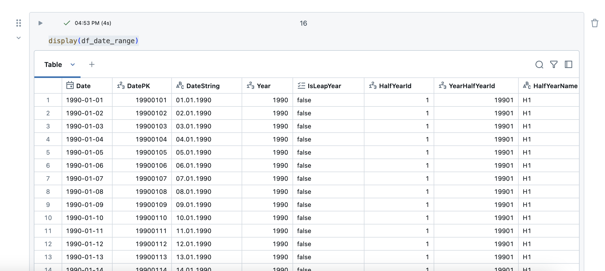
The content of the dataframe looks good.

Now I will create the dataframe for the time dimension.

1

df_time_range_minutes, time_columns = expand_date_to_datetime_table(df_date=df_date_range, resolution_in_seconds=60)

So that the two tables for time and date can be joined together later, I create a mapping table, which I can create from the following dataframe.

1
2
3


date_timestamp_columns = ["DateUtcFK", "TimestampStartUtc", "WeekTimePK"]

df_mapping_minutes = df_time_range_minutes.select(date_timestamp_columns)

In the following function, I make the final filtering for the dataframe for the time dimension.

1
2
3
4
5
6
7
8


week_time_filter_query = f"Year=year('{start_date}') AND Month=month('{start_date}')"

df_time_minutes = (df_time_range_minutes
                  .filter(week_time_filter_query)
                  .select(["WeekTimePK", "WeekTime", "WeekTimeDuration", "DayTimeDuration"]+time_columns)
                  .drop('TimestampPK', 'TimestampStartUtc')
                  .distinct()
                )

Now the dataframes are created, have the desired form and the data can be saved in the tables. When writing, I use the “overwriteSchema” option with the ulterior motive that the tables can be recreated by simply running this notebook again.

1

df_date_range.write.format("delta").mode("overwrite").option("overwriteSchema", "true").saveAsTable(date_table)

1

df_time_minutes.write.format("delta").mode("overwrite").option("overwriteSchema", "true").saveAsTable(time_minute_table)

1

df_mapping_minutes.write.format("delta").mode("overwrite").option("overwriteSchema", "true").saveAsTable(mapping_minute_table)

I create a view so that the time and date dimensions can be combined with each other. I join all the tables together in the view.

 1
 2
 3
 4
 5
 6
 7
 8
 9
10
11
12
13
14
15
16
17
18
19
20
21
22
23
24
25
26
27
28
29
30
31
32
33
34
35
36
37
38
39
40
41
42
43
44
45
46
47
48
49
50
51
52
53
54
55
56
57
58
59
60
61
62
63
64
65
66
67
68
69
70
71
72
73
74
75
76
77
78
79
80
81
82
83
84
85
86
87
88
89


sql = f"""
CREATE OR REPLACE VIEW {catalog}.silver.vw_dim_date_minute AS
  SELECT
    dd.Date,
    dd.DatePK,
    dd.DateString,
    dd.Year,
    dd.IsLeapYear,
    dd.HalfYearId,
    dd.YearHalfYearId,
    dd.HalfYearName,
    dd.YearHalfYear,
    dd.Quarter,
    dd.YearQuarterId,
    dd.YearQuarter,
    dd.QuarterShortname,
    dd.YearMonthId,
    dd.Month,
    dd.MonthName,
    dd.MonthNameShort,
    dd.MonthNameDe,
    dd.MonthNameShortDe,
    dd.MonthNameFr,
    dd.MonthNameShortFr,
    dd.MonthNameIt,
    dd.MonthNameShortIt,
    dd.WeekIdIso,
    dd.WeekOfYearIso,
    dd.WeekOfYearIsoName,
    dd.YearWeekOfYearIso,
    dd.DayName,
    dd.DayNameShort,
    dd.DayNameDe,
    dd.DayNameShortDe,
    dd.DayNameFr,
    dd.DayNameShortFr,
    dd.DayNameIt,
    dd.DayNameShortIt,
    dd.DayOfYear,
    dd.Day,
    dd.DayOfWeekUs,
    dd.DayOfWeekIso,
    dd.IsWeekDay,
    dd.IsLastDayOfMonth,
    dd.LastDayOfMonth,
    dd.MonthDay,
    dd.StartOfWeekUs,
    dd.StartOfWeekIso,
    dd.EndOfWeekUs,
    dd.EndOfWeekIso,
    dd.IsHoliday,

    tm.WeekTimePK,
    tm.WeekTime,
    tm.WeekTimeDuration,
    tm.DayTimeDuration,
    tm.TimePK,
    tm.Time,
    tm.TimeString,
    tm.TimeHour,
    tm.TimeMinute,
    tm.TimeSecond,
    tm.AmPm,
    tm.TimeSecondId,
    tm.TimeMinuteId,
    tm.IsWindow5MinuteStart,
    tm.Window5MinuteId,
    tm.Window5MinuteName,
    tm.IsWindow10MinuteStart,
    tm.Window10MinuteId,
    tm.Window10MinuteName,
    tm.IsWindow15MinuteStart,
    tm.Window15MinuteId,
    tm.Window15MinuteName,
    tm.IsWindow20MinuteStart,
    tm.Window20MinuteId,
    tm.Window20MinuteName,
    tm.IsWindow30MinuteStart,
    tm.Window30MinuteId,
    tm.Window30MinuteName,
    tm.IsWindow60MinuteStart,
    tm.Window60MinuteId,
    tm.Window60MinuteName

  FROM {catalog}.silver.dim_date AS dd
  LEFT OUTER JOIN {catalog}.silver.dim_mapping_minute AS mm ON dd.DatePK = mm.DateUtcFK
  LEFT OUTER JOIN {catalog}.silver.dim_time_minute AS tm ON mm.WeekTimePK = tm.WeekTimePK
"""
spark.sql(sql).display()

This view has all entries from the start date to the end date in an interval of one minute. If you need larger intervals, I have created additional views that only contain the corresponding time windows. This can be done relatively easily by filtering accordingly.

1
2
3
4
5
6


sql = f"""
CREATE OR REPLACE VIEW {catalog}.silver.vw_dim_date_5_minute AS
SELECT * FROM {catalog}.silver.vw_dim_date_minute
WHERE IsWindow5MinuteStart = true
"""
spark.sql(sql).display()

1
2
3
4
5
6


sql = f"""
CREATE OR REPLACE VIEW {catalog}.silver.vw_dim_date_10_minute AS
SELECT * FROM {catalog}.silver.vw_dim_date_minute
WHERE IsWindow10MinuteStart = true
"""
spark.sql(sql).display()

1
2
3
4
5
6


sql = f"""
CREATE OR REPLACE VIEW {catalog}.silver.vw_dim_date_15_minute AS
SELECT * FROM {catalog}.silver.vw_dim_date_minute
WHERE IsWindow15MinuteStart = true
"""
spark.sql(sql).display()

1
2
3
4
5
6


sql = f"""
CREATE OR REPLACE VIEW {catalog}.silver.vw_dim_date_20_minute AS
SELECT * FROM {catalog}.silver.vw_dim_date_minute
WHERE IsWindow20MinuteStart = true
"""
spark.sql(sql).display()

1
2
3
4
5
6


sql = f"""
CREATE OR REPLACE VIEW {catalog}.silver.vw_dim_date_30_minute AS
SELECT * FROM {catalog}.silver.vw_dim_date_minute
WHERE IsWindow30MinuteStart = true
"""
spark.sql(sql).display()

1
2
3
4
5
6


sql = f"""
CREATE OR REPLACE VIEW {catalog}.silver.vw_dim_date_60_minute AS
SELECT * FROM {catalog}.silver.vw_dim_date_minute
WHERE IsWindow60MinuteStart = true
"""
spark.sql(sql).display()

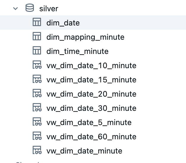
Now I have various tables and views in the Silver schema that can be used for the analyses.

These views and tables can now be used to build specific dimensions in the Gold Layer. For example, do I only need German and English languages in a dashboard in a much smaller time period and a 5-minute time window? No problem, I read out the corresponding view vw_dim_date_5_minute, filter the corresponding columns that I want to use and create a new view in the gold schema. In this way, any date and time dimensions can be generated from the Silver objects.

And here is the result. The dim_date table looks like this:

The table dim_time_minute:

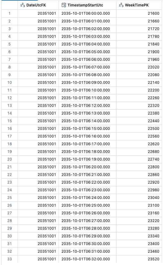
The mapping table:

Last but not least, the view, where date and time are joined:

Create a Job in Databricks

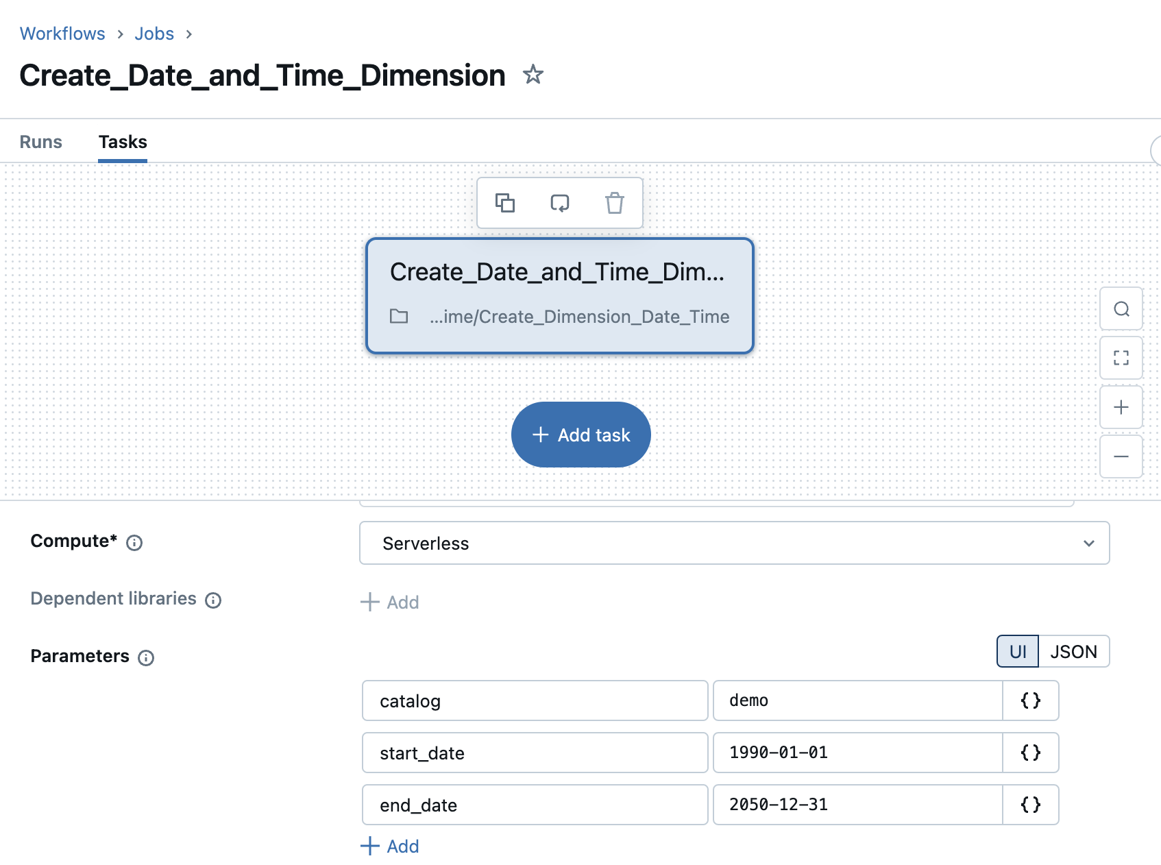
The notebook can be executed very well in a job if I want to generate the dimensions again later.

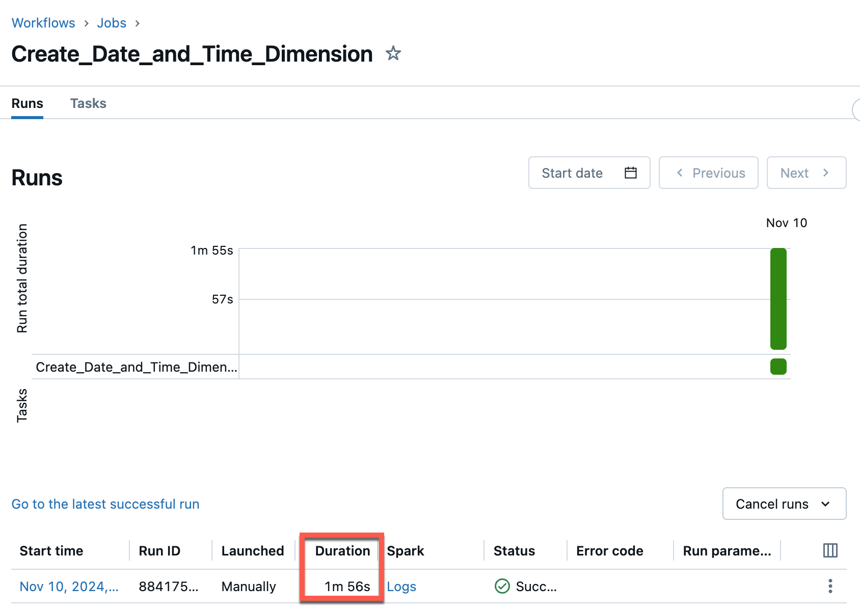
The execution of the job only takes less than 2 minutes with Serverless Compute.

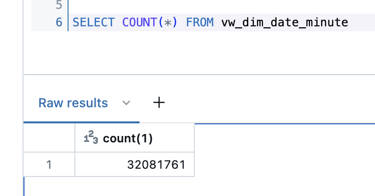
The generated view has a row count of over 32 million entries.

Considerations on the range of the date dimension

In my example, I have specified a very large range of 60 years. With Serverless Compute it is no problem to generate these dimensions. If the range is very large, you don’t have to generate the tables again. However, you could also argue that it is overkill because I certainly don’t have data in the full range. Here, for example, you could have the date dimension regenerated regularly with a start date that only goes into the past as long as you have data. And the end date would then only be 1 or 2 years into the future.

Create date and time dimensions only in the date range of a target table

Let’s say I want to build a report for a certain table and then make the corresponding date and time dimension only as large as the earliest and latest date in the table.

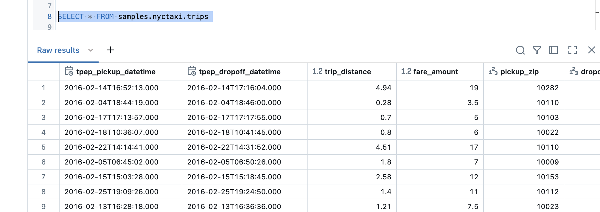
As an example I take the example table of NY City Taxi Trips.

The table has 2 date columns, one for Pickup Time and one for DropOff Time. If I look at when the first date is, then it is January 1, 2016.

The most recent date is 29.February 2016.

So I would only have to cover a time range of 2 months to create the analyses.

I rewrite the notebook accordingly. I don’t enter the start and end date as the widget, but the target table and date column.

1
2
3


dbutils.widgets.text('catalog', 'demo', 'Catalog')
dbutils.widgets.text('source_table', 'samples.nyctaxi.trips', 'Source Table')
dbutils.widgets.text('date_column', 'tpep_pickup_datetime', 'Date Column')

Again, save these in variables.

1
2
3


catalog       = dbutils.widgets.get('catalog')
source_table  = dbutils.widgets.get('source_table')
date_column   = dbutils.widgets.get('date_column') 

Then I get the minimum date from the source table for the corresponding column. To be on the safe side, I subtract an additional day so that I have all the dates for sure.

1
2
3
4
5


sql = f"""
      SELECT DATE_SUB(DATE(MIN({date_column})), 1) AS start_date FROM {source_table}
"""
df_start_date = spark.sql(sql)
start_date = df_start_date.collect()[0]['start_date']

I then do the same for the end date. Here too, an additional day as security.

1
2
3
4
5


sql = f"""
    SELECT DATE_ADD(DATE(MAX({date_column})), 1) AS end_date FROM {source_table}
"""
df_end_date = spark.sql(sql)
end_date = df_end_date.collect()[0]['end_date']

I name the corresponding tables according to the source table.

 1
 2
 3
 4
 5
 6
 7
 8
 9
10


date_table            = f'{catalog}.silver.dim_date_{source_table.replace(".", "_")}'
time_minute_table     = f'{catalog}.silver.dim_time_minute_{source_table.replace(".", "_")}'
mapping_minute_table  = f'{catalog}.silver.dim_mapping_minute_{source_table.replace(".", "_")}'

print(f'Create Dimension Tables for Date and Time')
print(f'Timerange: {start_date} to {end_date}')
print(f'Create the following tables: ')
print(f'{date_table}')
print(f'{time_minute_table}')
print(f'{mapping_minute_table}')

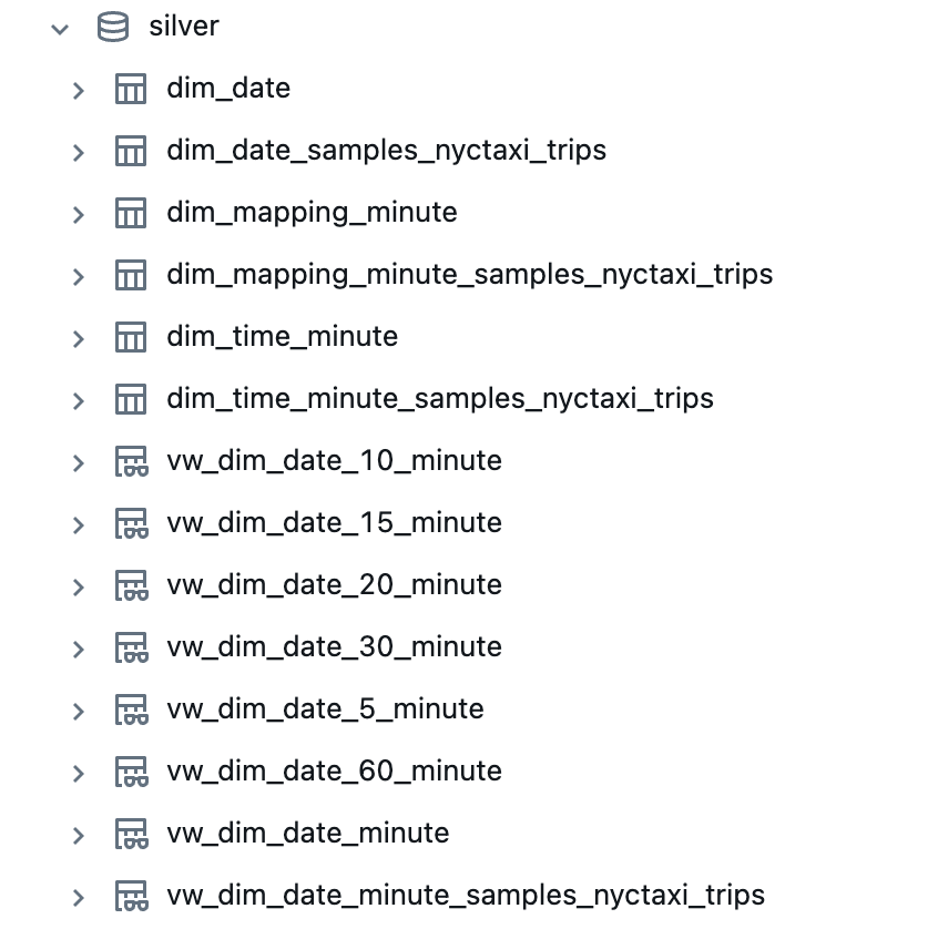
I now have these customized tables in my Silver schema.

As you can see, these consume much less storage.

Conclusion

With Databricks and a bit of PySpark code, you can create very useful date and time dimensions that are extremely flexible and customized to your needs. My code are examples, which can of course be extended further. I provide the code on my Github repo: https://github.com/stefanko-ch/Databricks_Dojo/tree/main/Dimension_Date_Time

If anyone has any suggestions or ideas as to which other columns could be included in the Date or Time dimension, I would be delighted to receive any feedback and am open to suggestions! Of course, general feedback is also welcome.