In this article I describe how to load data from recurring full snapshots with Delta Live Tables relatively easily and elegantly into a bronze table without the amount of data exploding.

Introduction

In many data integration projects, it is not always easy to efficiently read data from source systems. Ideally, we would access the source system’s Change Data Capture (CDC) directly in order to capture only the actual changes since the last retrieval. This means that the source system indicates which records are new (insert), which records have changed (update) and which records have been deleted (delete). This significantly reduces the amount of data to be processed and enables almost real-time synchronisation. However, CDC mechanisms are not available in all systems. Older ERP systems, proprietary databases or external APIs in particular often only offer one way to retrieve the data: via periodic full snapshots.

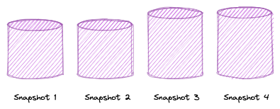
This means that the entire relevant dataset, whether a few megabytes or several gigabytes in size, is exported as a complete copy at regular intervals.

A full snapshot always contains the current status of the data at a specific point in time. There is no differentiation between newly added, changed or deleted data records. Instead, you simply receive a snapshot of the entire table, hence the name snapshot.

This brings with it several challenges:

Large amounts of data: The entire table is exported each time, even if only a small part of the data has changed. This can lead to high memory consumption and long loading times.

No change tracking: Because it is always a complete copy, there is no direct information about which rows are new, which have changed or which have been deleted.

Efficient processing required: In order to get a grip on the volume of data, strategies must be developed that only save relevant changes and avoid redundancies.

The bad news first: The data volume of the raw data cannot be reduced. The full snapshots still have to be saved and processed, as we have no way of retrieving only the changes directly from the source.

But there is also good news: we can save storage space and compute in the next steps of the Medallion architecture. By cleverly processing the full snapshots with Delta Live Tables, we can simulate a change data capture approach. This means that we only save the actual changes in the Silver and Gold layers and avoid redundant data - which leads to significantly more efficient memory and performance utilisation.

Databricks as a platform and Delta Live Tables (DLT) as a framework

I use Databricks as the platform in this example. Databricks is a unified, open analytics platform for building, deploying, sharing, and maintaining enterprise-grade data, analytics, and AI solutions at scale. The Databricks Data Intelligence Platform integrates with cloud storage and security in your cloud account, and manages and deploys cloud infrastructure on your behalf. More information about Databricks can be found here: https://docs.databricks.com/aws/en/introduction/

DLT is a declarative framework designed to simplify the creation of reliable and maintainable extract, transform, and load (ETL) pipelines. You specify what data to ingest and how to transform it, and DLT automates key aspects of managing your data pipeline, including orchestration, compute management, monitoring, data quality enforcement, and error handling.

DLT is built on Apache Spark, but instead of defining your data pipelines using a series of separate Apache Spark tasks, you define streaming tables and materialized views that the system should create and the queries required to populate and update those streaming tables and materialized views.

More information about Delta Live Tables can be found here: https://learn.microsoft.com/de-de/azure/databricks/dlt/

Simulation of full snapshots: How to create test data

Before I can get down to the actual processing, I first need a realistic data basis. This means that I will generate periodic full snapshots, i.e. complete table copies that are exported at regular intervals. I have created a notebook for this purpose. I use the Python package faker to create the fake data: https://faker.readthedocs.io/

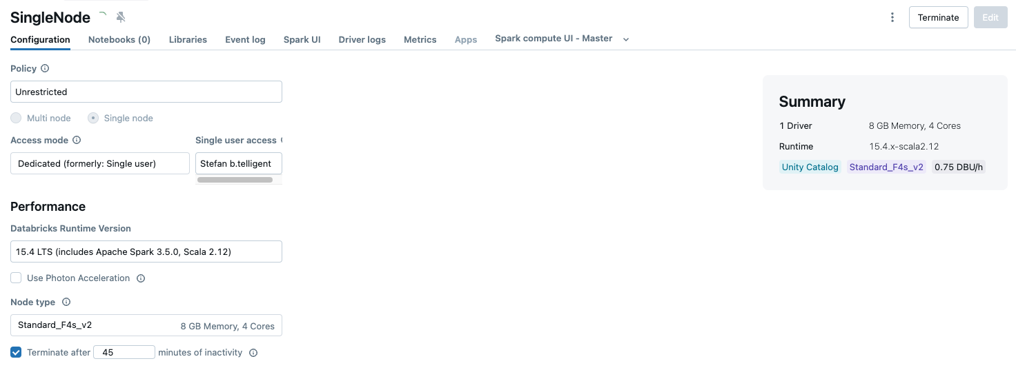
No large cluster is needed to create the test data; I create a small single node, which is relatively inexpensive. Alternatively, you could also use serverless.

Faker is not installed on the cluster by default and must therefore be installed first.

1

%pip install faker

In the subsequent code, I need various other libraries, which I import and then I create an instance of Faker.

1
2
3
4
5
6
7
8
9

import re
import uuid
import os
import pandas as pd
from pyspark.sql.functions import current_timestamp, sha2, concat, lit, col, udf
from pyspark.sql.types import StringType
from datetime import datetime, timedelta
from faker import Faker
fake = Faker()

I use dbutils to create a widget that can be used to pass user input. I use this so that I can define a catalogue, which I use for my example. I also need a start date for the first snapshot.

1
2

dbutils.widgets.text("catalog_name", "demo", "Catalog, where the data will be stored.")
dbutils.widgets.text("first_snapshot_date", "2025-03-01", "Date, when the first snapshot was taken.") 

In the next step, I define the volume in which I want to save the snapshots, as well as a table in which I write the test data. This table simulates the source system, i.e. a table from an OLTP source system.

A snapshot is to be created for each execution of the notebook. I want to simulate that a full snapshot is taken every day. To do this, I have to simulate a mechanism in my notebook that each run of the notebook should take place on a subsequent day. To do this, I use a CSV file in which I write the date. During the following run, the last date is read out, incremented by one and written back again. If I want to start the test again, I can simply delete the CSV file.

1
2
3
4
5
6

catalog_name = dbutils.widgets.get("catalog_name")
first_snapshot_date = datetime.strptime(dbutils.widgets.get("first_snapshot_date"), "%Y-%m-%d")

source_volume = f"/Volumes/{catalog_name}/source/raw"
customer_source_table = f"{catalog_name}.source.customer"
date_csv_path = f"/Volumes/{catalog_name}/source/raw/snapshot_dates.csv"

Now I create a function that creates the snapshot timestamp and returns the number of the iteration. The iteration is the number of times this notebook has already been executed. I derive the iteration from the row number in the CSV file.

The remaining logic of the function is relatively simple. If the CSV file does not exist, take the date from the widget, create the timestamp and save the timestamp in the CSV. If the CVS file already exists, read the last timestamp, increase the date by one day and add the new timestamp to the file.

 1
 2
 3
 4
 5
 6
 7
 8
 9
10
11
12
13
14
15
16
17
18
19
20
21
22
23
24
25
26
27
28
29
30
31
32
33
34
35
36
37
38
39
40
41
42
43
44
45
46
47
48
49
50
51

def update_snapshot_date(date_csv_path: str, first_snapshot_date: datetime) -> tuple:
    """
    Updates the snapshot date in the given CSV file.

    - If the file exists, it reads the latest snapshot date, increments it by one day, and appends it.
    - If the file does not exist, it initializes it with the first snapshot date.

    Parameters:
        date_csv_path (str): Path to the snapshot CSV file.
        first_snapshot_date (datetime): The initial snapshot date to use if the file does not exist.

    Returns:
        tuple: (datetime, int) - The newly added snapshot date and the row count (iteration).
    """

    # Check if the CSV file exists
    if os.path.exists(date_csv_path):
        # Load the existing CSV file
        existing_df = pd.read_csv(date_csv_path, dtype=str)  # Read as string to prevent automatic type conversion

        # Convert the column to datetime format
        existing_df["snapshot_date"] = pd.to_datetime(existing_df["snapshot_date"]).dt.date  # Keep only the date part

        # Get the latest snapshot date
        latest_snapshot_date = existing_df["snapshot_date"].max()

        # Increment the date by one day
        snapshot_timestamp = latest_snapshot_date + timedelta(days=1)

        # Append the new timestamp (ensure it's a string)
        new_entry = pd.DataFrame({"snapshot_date": [snapshot_timestamp.isoformat()]})
        updated_df = pd.concat([existing_df, new_entry], ignore_index=True)

        # Save the updated CSV file (force writing only date format)
        updated_df.to_csv(date_csv_path, index=False, date_format='%Y-%m-%d')

        # Get the row count (iteration)
        iteration = len(updated_df)

        print(f"New snapshot timestamp {snapshot_timestamp} saved. Iteration: {iteration}")
    else:
        # If the file does not exist, create it with the first snapshot date
        snapshot_timestamp = first_snapshot_date
        df = pd.DataFrame({"snapshot_date": [snapshot_timestamp.isoformat()]})  # Store as string
        df.to_csv(date_csv_path, index=False)

        # Since it's the first row, iteration = 1
        iteration = 1
        print(f"Snapshot timestamp {snapshot_timestamp} saved. Iteration: {iteration}")

    return snapshot_timestamp, iteration  # Return both values

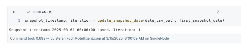
If I now call the function, I get the snapshot timestamp and the iteration.

It has created a CSV file in the volume.

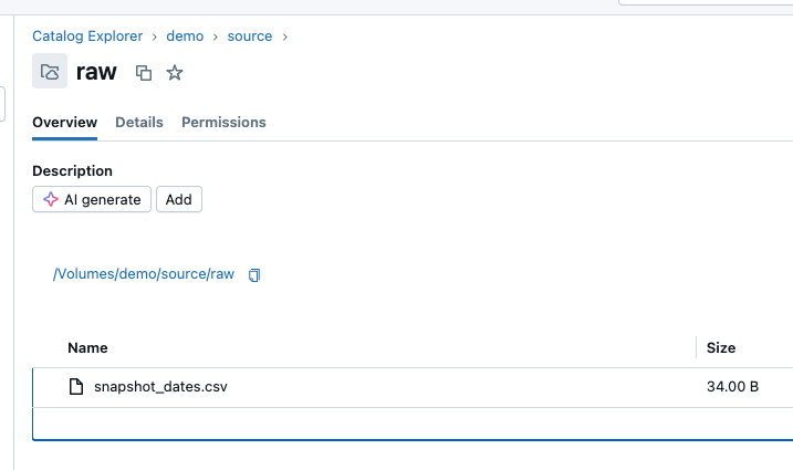
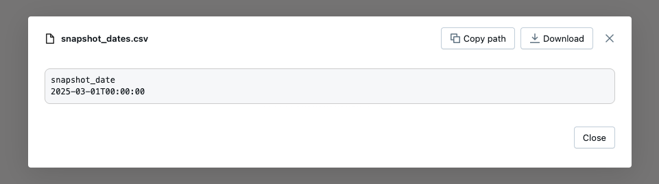
The contents look as expected.

The catalogue already exists in my environment, the remaining resources must be created if they do not already exist.

1
2
3

spark.sql(f"CREATE SCHEMA IF NOT EXISTS {catalog_name}.source")
spark.sql(f"CREATE SCHEMA IF NOT EXISTS {catalog_name}.bronze")
spark.sql(f"CREATE VOLUME IF NOT EXISTS {catalog_name}.source.raw")

I now use Faker to generate the test data and save it in a dataframe. For the test data, I select personal data, which should simulate a customer table. I generate 5 data records, which is sufficient for my example.

 1
 2
 3
 4
 5
 6
 7
 8
 9
10
11
12
13

# Create a list of fake person data
data = []
for i in range(5):
    primary_key = str(uuid.uuid4()) # Generate a unique primary key
    name = fake.first_name()
    surname = fake.last_name()
    dob = fake.date_of_birth()
    age = fake.random_int(min=18, max=99)

    data.append((primary_key, name, surname, dob, age))

# Create a DataFrame
df_customer_delta = spark.createDataFrame(data, ['primary_key', 'name', 'surname', 'date_of_birth', 'age'])

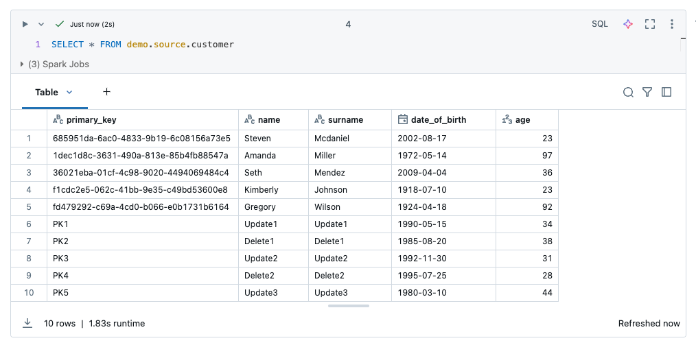
The generated data then looks like this:

I have deliberately refrained from creating many columns so that it is not confusing. An important column is ‘primary_key’, which is the unique key with which a customer can be identified.

The data is still in the dataframe, i.e. in the memory of the Spark Cluster. I now write this to the customer table. To make it easier to compare certain data later, I will generate an additional 5 data records and write them to the table. However, this only happens during the first run; this should not happen during the subsequent runs of the notebook. I use the variable of the iteration for this.

 1
 2
 3
 4
 5
 6
 7
 8
 9
10
11

if iteration == 1:
    print("Insert additional data")
    spark.sql(f"""INSERT INTO {customer_source_table} VALUES
        ('PK1', 'Update1', 'Update1', '1990-05-15', 34),
        ('PK2', 'Delete1', 'Delete1', '1985-08-20', 38),
        ('PK3', 'Update2', 'Update2', '1992-11-30', 31),
        ('PK4', 'Delete2', 'Delete2', '1995-07-25', 28),
        ('PK5', 'Update3', 'Update3', '1980-03-10', 44);
        """)
else: 
    print("No additional data to insert.")

As you can see, I did not generate this data with Faker, but defined it myself. For the sake of simplicity, I have not used a GUID for the primary keys, but simple strings. I have also entered the planned operation for the name and surname columns. An update is to be performed on PK1, a delete on PK2, and so on.

I will simulate updates and deletes for later loads. In the 2nd run, an update is to be made, for this I have created the following code:

1
2
3
4
5
6
7
8
9

if iteration == 2:
    print("Will do Update #1")
    spark.sql(f"""
    UPDATE {customer_source_table} 
    SET name = 'UPDATED', surname = 'UPDATED'
    WHERE primary_key = 'PK1';
    """)
else:
    print("Nothing to do")

Then one run later comes a Delete:

1
2
3
4
5
6
7
8

if iteration == 3:
    print("Will do Delete #1")
    spark.sql(f"""
    DELETE FROM {customer_source_table} 
    WHERE primary_key = 'PK2';
    """)
else:
    print("Nothing to do")

For the next two runs, an update and a delete are built in. But more on this later.

The content of the source table now looks like this.

I now want to write the contents of this table to a volume as a snapshot. To do this, I read the data into a dataframe.

1

df_customer_snapshot = spark.read.table(f"{customer_source_table}")

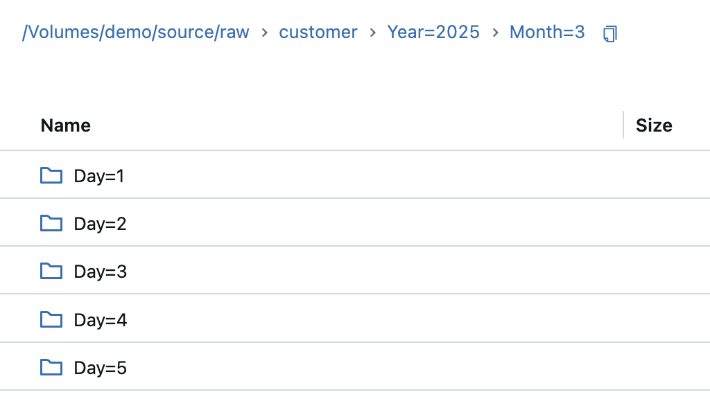
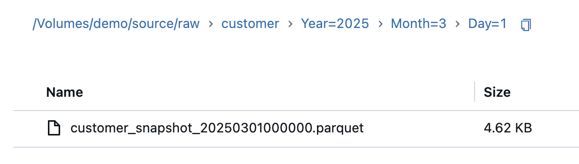
I will use Parquet as the file format for the snapshots. If I were to write this myself using the Spark method, it would generate a folder with several Parquet files, as Spark is optimised for parallelisation. With Pandas, I can write this as a single file, so I convert the PySpark dataframe into a Pandas dataframe. In addition, I create a partitioning in the target directory according to year, month and day, just as it would be done in practice. The current timestamp is entered as a string in the file name of the file so that the file name looks like this: customer_snapshot_20250301000000.parquet. This allows you to recognise later when a snapshot was created.

 1
 2
 3
 4
 5
 6
 7
 8
 9
10
11
12
13
14
15
16

timestamp_string = snapshot_timestamp.strftime("%Y%m%d%H%M%S")
year    = snapshot_timestamp.year
month   = snapshot_timestamp.month
day     = snapshot_timestamp.day

output_path = os.path.join(
                            source_volume, 
                            "customer/",
                            f"Year={year}/Month={month}/Day={day}/"
                            )
file_name = f"customer_snapshot_{timestamp_string}.parquet"

os.makedirs(output_path, exist_ok=True)

pdf_customer_snapshot = df_customer_snapshot.toPandas()
pdf_customer_snapshot.to_parquet(f"{output_path}{file_name}")

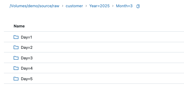
The result in the volume then looks like this:

Loading data with Delta Live Tables

Raw data in a volume can be stored relatively easily in a streaming table using Delta Live Tables. At the beginning I will show you how not to do it, i.e. simply save all data from the source in a Bronze Table. I call the table ‘customer_append’ because it is append only. This way, the amount of data explodes over time and the processing of the pipeline becomes slower with each execution.

I create a new notebook for the Delta Live Table Pipeline. I create a new streaming table and read in the Parquet files as a stream using Databricks Autoloader. The schema should adapt to the source data, so I set the ‘mergeSchema’ option to true.

 1
 2
 3
 4
 5
 6
 7
 8
 9
10
11
12
13
14
15
16
17
18

import dlt
table_name = "customer_append"

@dlt.table(
    name = table_name,
    comment = 'This is an append only table',
    table_properties = {"quality": "bronze"}
)

def build_table():
    df = (spark.readStream
                .format("cloudFiles")
                .option("cloudFiles.format", "parquet")
                .option("mergeSchema", "true")
                .load(f"/Volumes/demo/source/raw/customer/")
    )
    
    return df

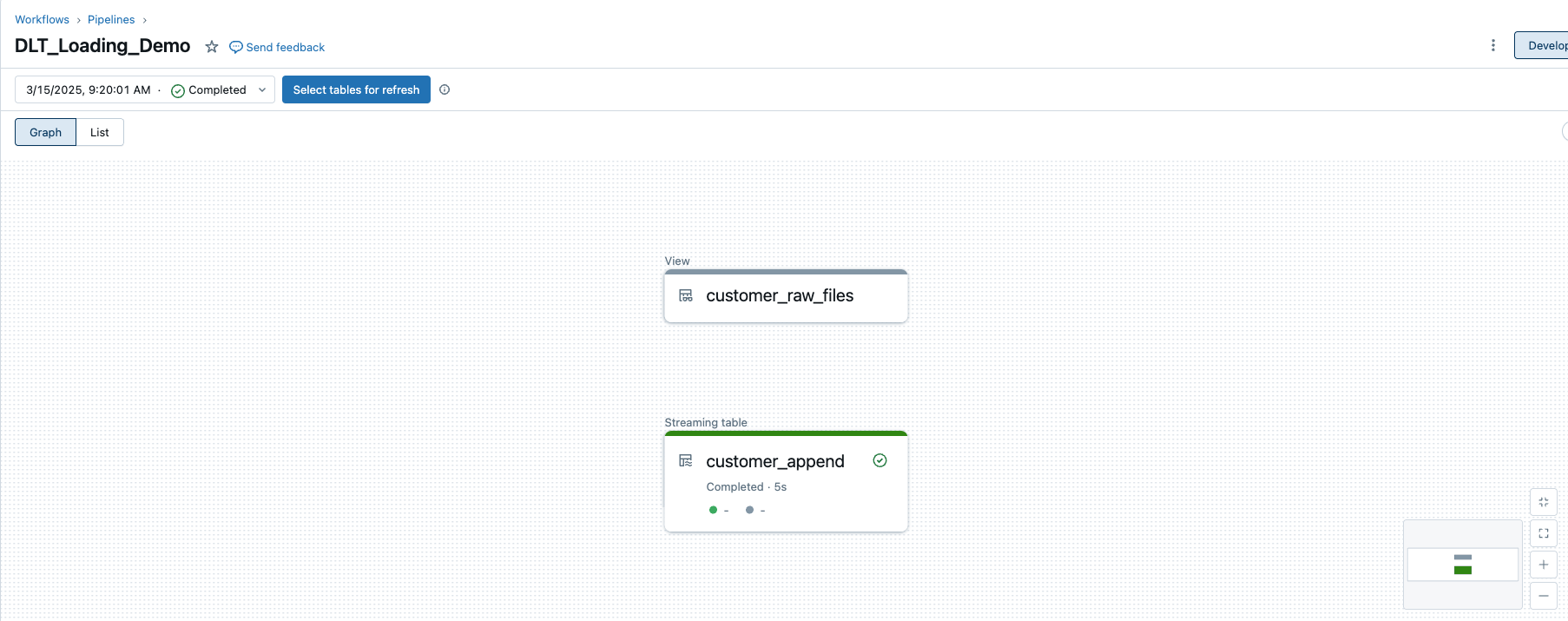
When I start the DLT for the first time, I get the following result:

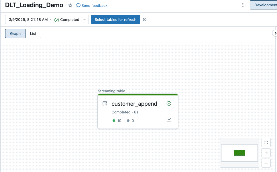
It has loaded all 10 rows from the Parquet file. The content of the Bronze table now looks like this:

I see 4 additional columns. The columns Year, Month and Day have been automatically taken over by Spark from the partitioning in the source directory. When Auto Loader infers the schema, a rescued data column is automatically added to your schema as _rescued_data. The rescued data column ensures that columns that don’t match with the schema are rescued instead of being dropped.

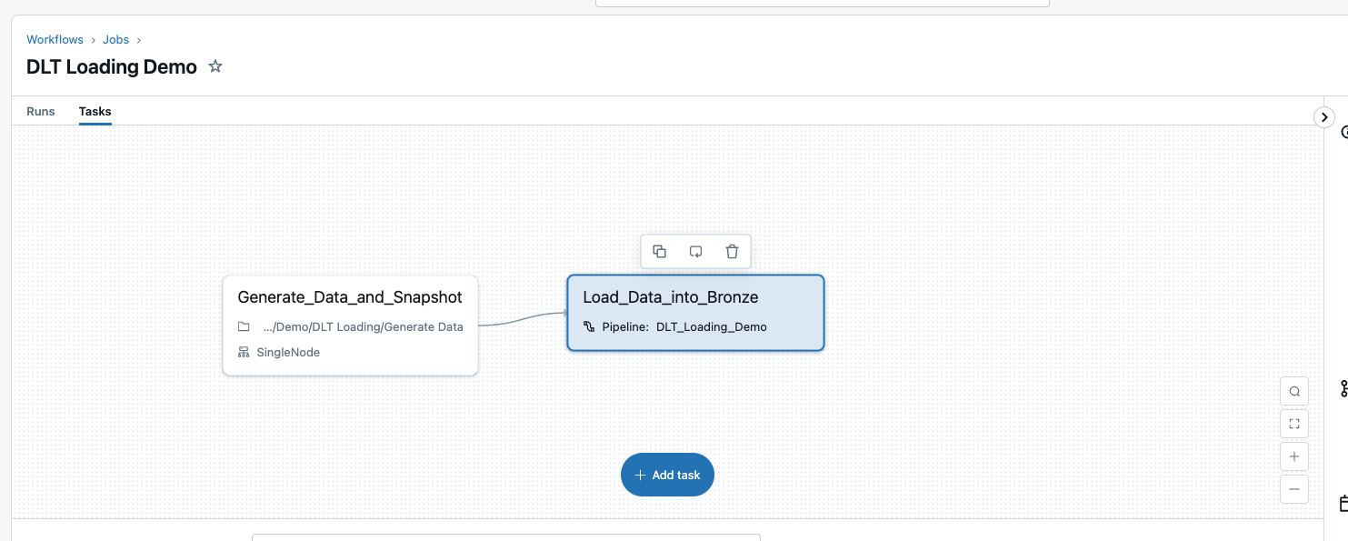
What happens now if I load in a 2nd snapshot? For this reason, I will run the notebook with the test data generation again and start the Deltas Live Table Pipeline immediately afterwards. To automate this a little, I will put the two steps into one job.

The append table now looks like this:

As is easy to see, we have a multiplication of the amount of data. It is also not clear when which record was loaded into the table. It is also not clear that the record with the primary key ‘PK1’ has changed. I set this in the first notebook so that the name and surname are changed.

As this is a Bronze table, I do not change any columns. But what I do in Bronze is to enrich the data. For example, I want to know which raw file a data record came from so that I can trace it later. For this reason, I add the system metadata as an additional column. This can be done relatively easily by adapting the function for the streaming table. After the load, I make a select where I use * to select all columns and also the _metadata column:

1
2
3
4
5
6
7
8

								...........
                .load(f"/Volumes/demo/source/raw/customer/")
                .select(
                    "*"
                    , col('_metadata')
                )
    )
    return df

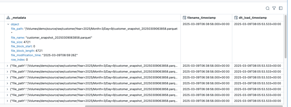
After this change, I have an additional column _metadata, which provides me with the following information:

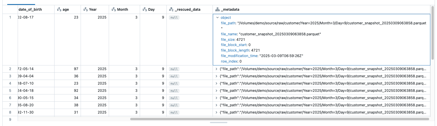
This metadata is file-specific metadata such as path, name, modification time. this is already very helpful. However, I would still like to know when the snapshot was created.

The timestamp of file_modification_time does not necessarily have to match the time when the snapshot was created. If the snapshot was created by another system and the files were subsequently loaded into the data lake, for example using Azure Data Factory, we already have a discrepancy. What happens if the snapshots are created, but for some reason the files cannot be copied to the data lake? If the copy pipeline for the delivery is then patched, the missing snapshots must be reloaded at the same time. If several snapshots are copied to the datalake at the same time, do they all have the same file_modification_time timestamp? Or only small differences? Even worse, the files may not be loaded onto the datalake in the correct order, depending on how the copy pipeline is set up. For this reason, I need the timestamp of the snapshot and cannot rely on the file modification timestamp.

I have saved the snapshot timestamp as a string in the file name. I will add this as an additional column to the dataframe.

1

df = df.withColumn("file_name", col("_metadata").getField("file_name"))

Using regex, I extract only the part of the name that contains the timestamp and convert it to a timestamp type in a second step.

1
2

df = df.withColumn("filename_timestamp_str", regexp_extract("file_name", r"(\d{14})", 1))
df = df.withColumn("filename_timestamp", to_timestamp("filename_timestamp_str", "yyyyMMddHHmmss"))

In addition, I would like to have a timestamp that tells me the time at which the DLT pipeline was executed. This can be realised using the function current_timestamp().

1

df = df.withColumn("dlt_load_timestamp", (current_timestamp()))

I needed the filename_timestamp_str and file_name columns for the intermediate steps. I no longer need them, as I can find this information in the metadata, so I delete them from the dataframe.

1
2

df = df.drop("filename_timestamp_str")
df = df.drop("file_name")

The complete code now looks like this:

 1
 2
 3
 4
 5
 6
 7
 8
 9
10
11
12
13
14
15
16
17
18
19
20
21
22
23
24
25
26
27
28
29
30
31
32
33
34
35
36
37

import dlt, re
from pyspark.sql.functions import col, to_date, regexp_replace, current_timestamp, regexp_extract, to_timestamp, date_format, concat, lit, max
from pyspark.sql.types import DateType, FloatType, StringType, IntegerType, StructType, StructField, LongType, TimestampType

table_name = "customer_append"

@dlt.table(
    name = table_name,
    comment = 'This is an append only table',
    table_properties = {"quality": "bronze"}
)

def build_table():
    df = (spark.readStream
                .format("cloudFiles")
                .option("cloudFiles.format", "parquet")
                .option("mergeSchema", "true")
                .load(f"/Volumes/demo/source/raw/customer/")
                .select(
                    "*"
                    , col('_metadata')
                )
    )
    # Add the filename by extracting it from _metadata.file_path
    df = df.withColumn("file_name", col("_metadata").getField("file_name"))

    # Extract timestamp using regex
    df = df.withColumn("filename_timestamp_str", regexp_extract("file_name", r"(\d{14})", 1))
    df = df.withColumn("filename_timestamp", to_timestamp("filename_timestamp_str", "yyyyMMddHHmmss"))

    df = df.withColumn("dlt_load_timestamp", (current_timestamp()))
    
    # drop unnecessary columns
    df = df.drop("filename_timestamp_str")
    df = df.drop("file_name")
    
    return df

I do a full refresh on the DLT and load the data in again. Then I have the following additional columns, which give me the corresponding insights:

The dlt_load_timestamp column now has the same value for all rows, as I have performed a full refresh. However, if the pipeline is executed after each delivery of the snapshots, then it is correct.

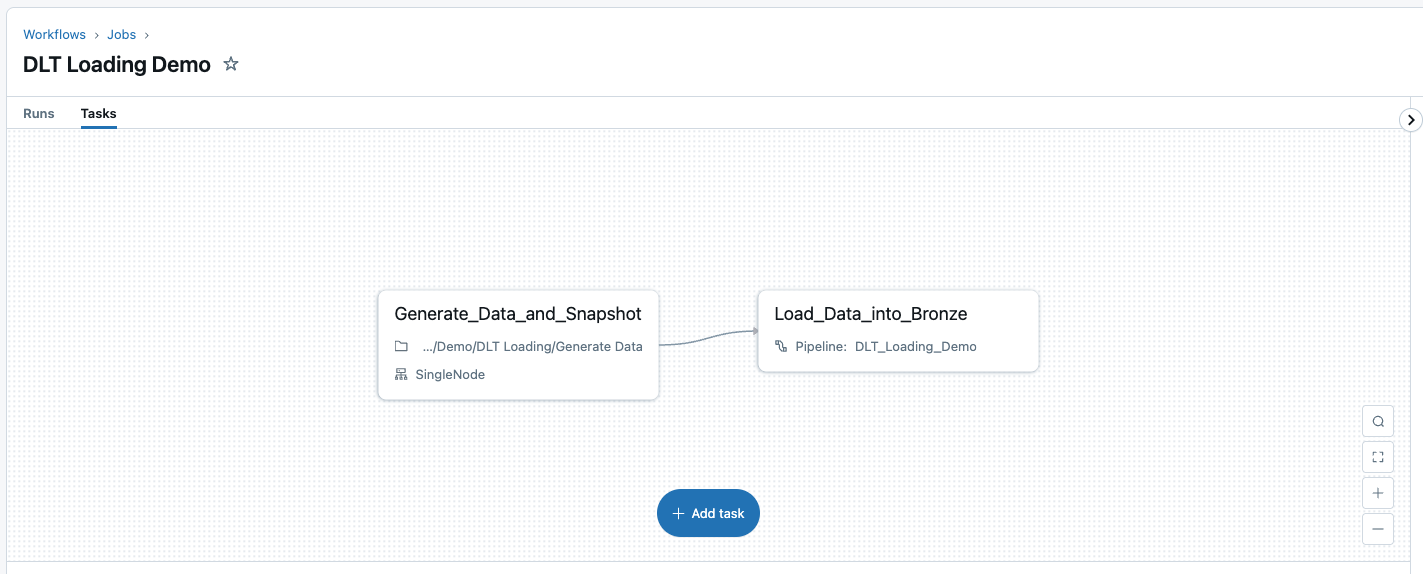
I now run the job 3 times in a row so that the data is generated and loaded immediately via DLT. But more about the timestamps and why they are important for the final solution later.

I have combined these two steps into one job so that I don’t have to manually run the notebook first and then start the DLT.

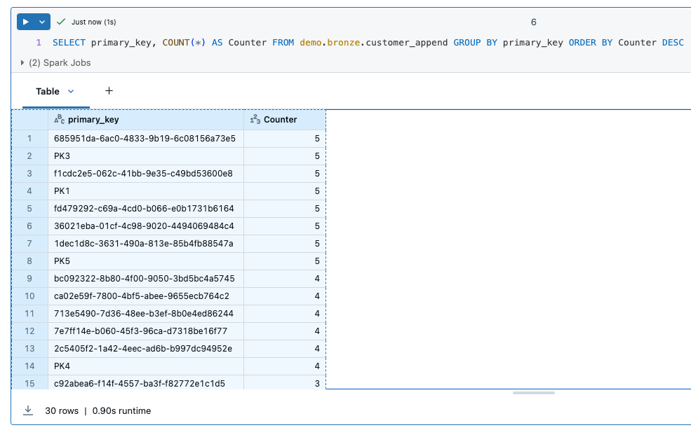
In total, I have loaded data from 5 snapshots.

And the bronze table now has a correspondingly large number of duplicates.

The question now is whether it makes sense to load all snapshots 1:1 into a bronze table. You generate a lot of data and still have to create a mechanism to filter out the updates and deletes from the huge data set. On the other hand, you can argue that if the data is in the bronze table, then the raw files can be archived and deleted.

From Append-Only to Latest-Records-Only

I can remember situations with customers where there were heated discussions about how to implement historisation. Various options were presented that were either costly, required a lot of computer resources and so on. Until it was discovered that historisation was not a business requirement at all. They would simply be happy if they could analyse the latest status of the data. So no over-engineering if the requirements are very simple.

This now means that we want to start the pipeline every day and overwrite the content of the bronze table with the last snapshot. This could actually be done relatively easily with 2 lines of SQL like this:

1
2
3

TRUNCATE TABLE your_catalog.your_schema.your_table;

INSERT INTO your_catalog.your_schema.your_table SELECT * FROM parquet.`/path/to/your_file.parquet`;

What remains is to recognise the path dynamically so that I can recognise the last Parquet file. I would also have problems with schema changes, as I would have to delete the table and recreate it. From my point of view, this is not a solution that I would like to pursue further.

From Latest-Records-Only to Change Tracking (CDC SCD1)

So that I don’t have to load every single record into the Bronze table, I have used merge functions in SQL in the past. Merge compares two data sets, inserts new records or updates records that have changed. However, some of these merge statements were quite complex, especially if you wanted to implement Slowly Changing Dimensions (SCD2). More information on Slowly Changing Dimensions can be found here: https://en.wikipedia.org/wiki/Slowly_changing_dimension

In Delta Live Table there is a simpler option than Merge, namely the functions of the APPLY CHANGES APIs. These functions can be used to realise Change Data Capture, more information can be found here: https://docs.databricks.com/aws/en/dlt/cdc

I would also like to use the Databricks autoloader with the CDC functionality. For this purpose, I create a view instead of a streaming table on the raw files and give it the same loading functionality as the streaming table. This means that the data is loaded using the autoloader when the view is called, but is not persisted. This means that the autoloader checkpoints are used.

The definition of the view looks like this:

 1
 2
 3
 4
 5
 6
 7
 8
 9
10
11
12
13
14
15
16
17
18
19
20
21
22
23
24
25
26
27
28
29
30
31

view_name = "customer_raw_files"

@dlt.view(
        name = view_name,
        comment = 'The purpose of this view is to use Auto-Loader to read the data from the datalake.',
    )
def build_view():
    df = (spark.readStream
                .format("cloudFiles")
                .option("cloudFiles.format", "parquet")
                .option("mergeSchema", "true")
                .load(f"/Volumes/demo/source/raw/customer/")
                .select(
                    "*"
                    , col('_metadata')
                )
    )
    # Add the filename by extracting it from _metadata.file_path
    df = df.withColumn("file_name", col("_metadata").getField("file_name"))

    # Extract timestamp using regex
    df = df.withColumn("filename_timestamp_str", regexp_extract("file_name", r"(\d{14})", 1))
    df = df.withColumn("filename_timestamp", to_timestamp("filename_timestamp_str", "yyyyMMddHHmmss"))

    df = df.withColumn("dlt_load_timestamp", (current_timestamp()))
    
    # drop unnecessary columns
    df = df.drop("filename_timestamp_str")
    df = df.drop("file_name")
    
    return df

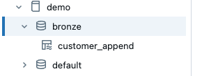
If I now start the DLT pipeline again, I see the new view.

However, the view is not persisted, i.e. it is only visible within the DLT pipeline and cannot be queried externally, for example in the Unity Catalogue. It does not appear in the Bronze Catalogue.

But we can use the view as a source for the CDC function. The definition for the new streaming table is very simple.

 1
 2
 3
 4
 5
 6
 7
 8
 9
10
11

cdc_table_scd1 = 'customer_cdc_scd1'

dlt.create_streaming_table(cdc_table_scd1)

dlt.apply_changes(
        target=cdc_table_scd1,
        source=view_name,
        keys=["primary_key"],
        sequence_by=col("filename_timestamp"),
        stored_as_scd_type = 1
    )

What we need here is the key with which the records can be compared, analogous to a merge statement. This can be a single column, such as the ‘primary_key’ column in my example. However, it can also be a list of columns if it is a composite key, i.e. a key that is made up of several columns.

The function must now have the information on how the respective records can be differentiated. In order for the data to be compared, the primary keys must be unique, as is the case with the merge statement. This differentiation is realised with a sequence. As I am loading data from different snapshots in my example, the filename_timestamp is a good choice. This allows the function to differentiate between different records with their primary key and the time.

Finally, we specify the SCD type, in our example it is type 1, which means that changes are overwritten and there is no historisation.

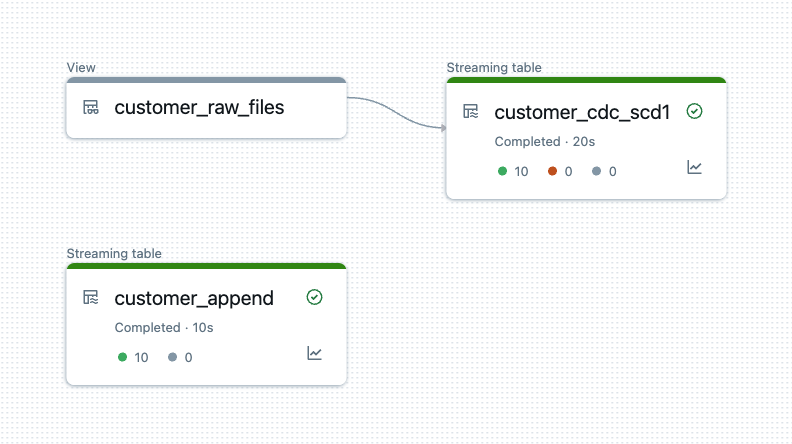
The extended DLT pipeline now looks like this.

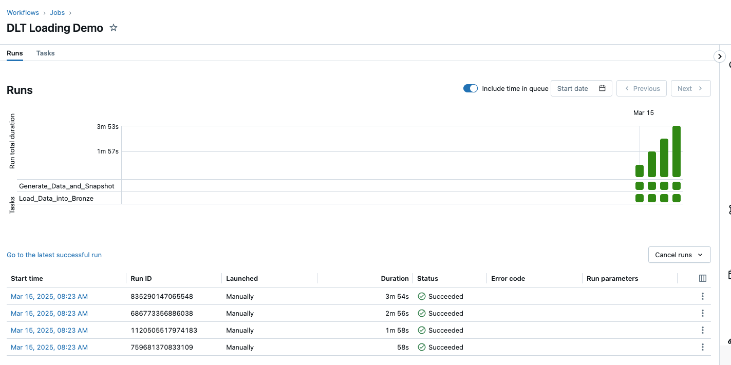
So that we can now understand the whole thing, I delete all snapshot data and the customer table and start from the beginning. I run the process a total of 5 times in succession. I have to do the first run manually. This means using the notebook to generate the data and then triggering a full_refresh in the DLT pipeline so that we no longer have the old data in it.

The job can then be executed 4 times.

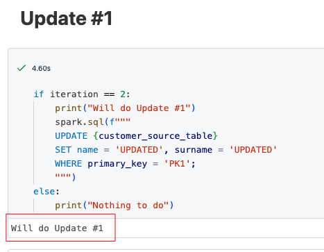
As I described at the beginning, update and delete operations are also carried out in the notebook runs in addition to the inserts. The following is an extract from the update run.

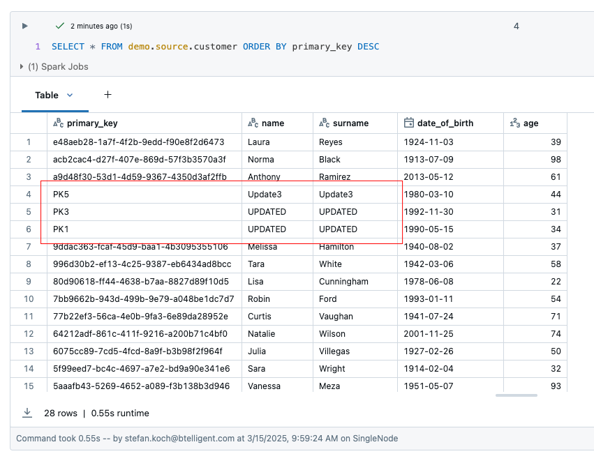
Now let’s take a look at the result. The source table customer has 28 rows. 2 rows were deleted, namely those with the primary key ‘PK2’ and ‘PK4’. The rows ‘PK1’ and ‘PK2’ were updated.

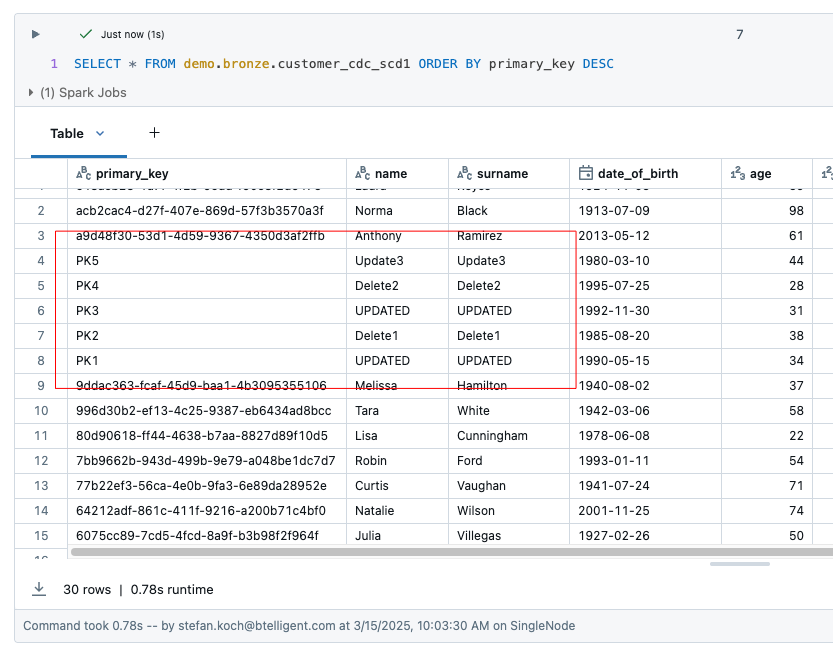
The table customer_cdc_scd1 has a total of 30 rows. You can see that the changes to PK1 and PK2 have been adopted, but the deletes have not been adopted. This means that PK2 and PK4 are still present in this table.

The deletes cannot be easily detected. According to the Databricks documentation, the source system would have to provide this information in order to recognise the deletes. This means that the dataset would have to contain an additional ‘Operation’ column in which the deletion process is flagged. The parameter apply_as_deletes would have to be defined in this way, as the following example shows.

 1
 2
 3
 4
 5
 6
 7
 8
 9
10

dlt.apply_changes(
  target = "target",
  source = "users",
  keys = ["userId"],
  sequence_by = col("sequenceNum"),
  apply_as_deletes = expr("operation = 'DELETE'"),
  apply_as_truncates = expr("operation = 'TRUNCATE'"),
  except_column_list = ["operation", "sequenceNum"],
  stored_as_scd_type = 1
)

From Change Tracking (CDC SCD1) to Change Tracking (CDC SCD2)

In addition to the streaming table with SCD1, I create one with SCD2. I change the parameter stored_as_scd_type to the value 2. The definition of the column now looks like this:

 1
 2
 3
 4
 5
 6
 7
 8
 9
10
11
12

cdc_table_scd2 = 'customer_cdc_scd2'

dlt.create_streaming_table(cdc_table_scd2)

dlt.apply_changes(
        target=cdc_table_scd2,
        source=view_name,
        keys=["primary_key"],
        sequence_by=col("filename_timestamp"),
        stored_as_scd_type = 2,
        track_history_except_column_list = ["_metadata", "filename_timestamp", "dlt_load_timestamp" ]
    )

As you can see, there is another parameter that I define, namely the ability to exclude columns from the comparison. As apply_changes checks all columns to see if there have been any changes, I have to exclude the columns that contain the metadata. Otherwise it would recognise an update with every run, even though nothing has changed in the source data.

Before I start the pipeline, I clean up the test setup again by deleting all files in the volume and the customer table.

The generated DLT pipeline now looks like this. I use the same view customer_raw_files for both SCD1 and SCD2.

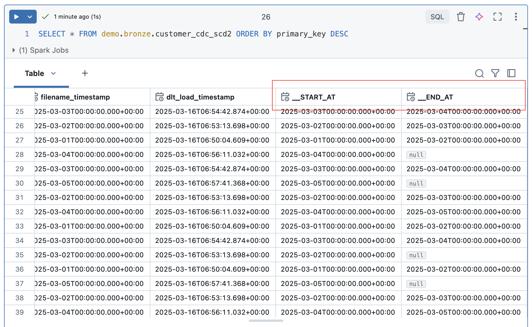
Now let’s take a look at the result of the table. After 5 runs, we have a total of 96 rows. As we are loading with SCD2, two additional columns START_AT and END_AT are added to the bronze table. These are used to define the validity of the rows. In other words, if a record has been deleted, it is not deleted from the Bronze Table, but the __END_AT date is set to indicate that it is no longer valid from the time of loading. During an update, the end time is also set and the new, changed value is added in a new row with a start date but without an end time. This means that all records that do not have an end time are valid values. So much for the theory…..

Let’s take a closer look at the rows that have been updated, i.e. the customers with the keys PK1 and PK3.

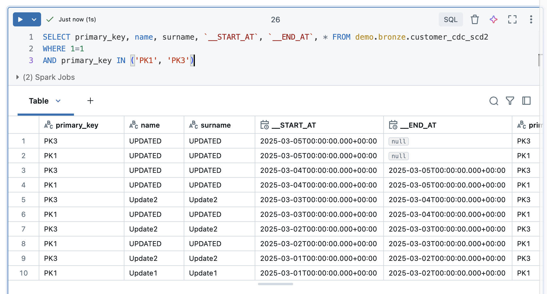
The updates were recorded correctly. Both values each have a valid entry without an end time at the start of the 5th iteration. The values in the 4 previous iterations were terminated with an end time.

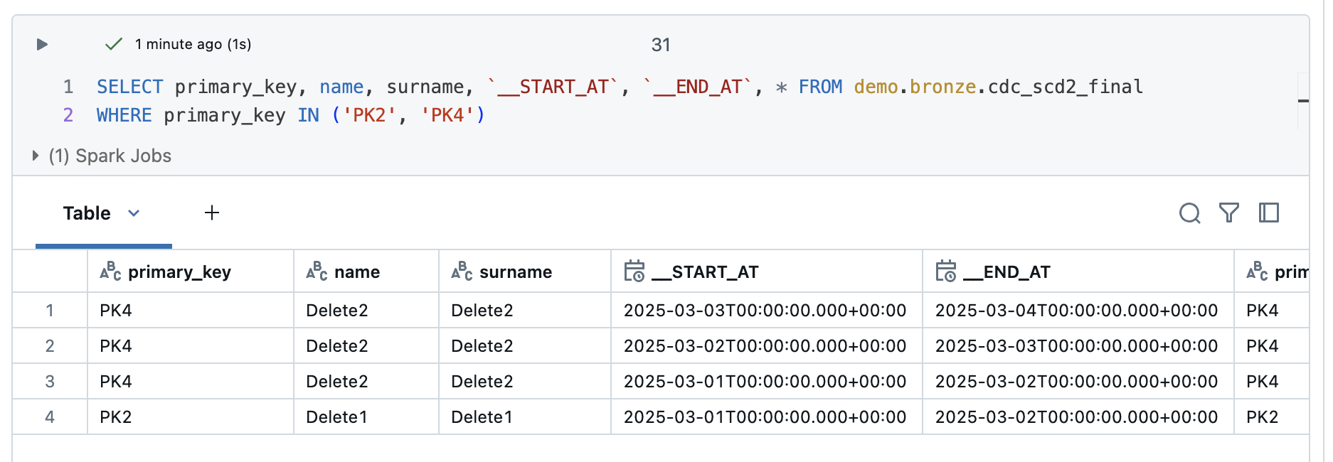
The deleted values of customer PK2 and PK4 are different. PK2 was deleted in the 3rd iteration and PK4 in the 5th iteration. However, these values are still entered as valid in the table.

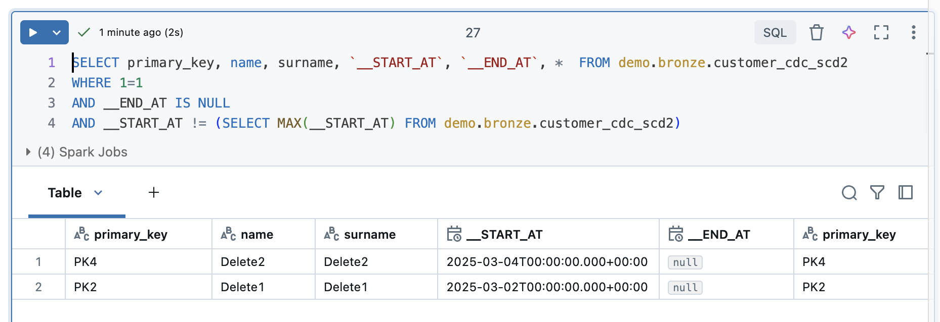
This is understandable, as the function requires an operation column to recognise these deletes. However, you can recognise a pattern for deleted values. The start time is reset for each iteration. This means that current values and those that have been changed always have the last start time. However, as the deleted records are no longer delivered, they remain in the table without an end time and without the start time being adjusted. If you filter according to these two criteria, the Deletes.

1
2
3
4

SELECT primary_key, name, surname, `__START_AT`, `__END_AT`, *  FROM demo.bronze.customer_cdc_scd2
WHERE 1=1
AND __END_AT IS NULL
AND __START_AT != (SELECT MAX(__START_AT) FROM demo.bronze.customer_cdc_scd2)

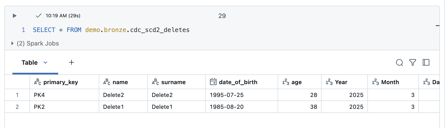
The result looks correspondingly good, PK2 and PK4 are now displayed.

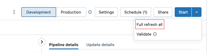
But what happens if I have to do a full refresh? To show this, I will do a full reflesh all to the Delta Live Tables and then take another look at the result.

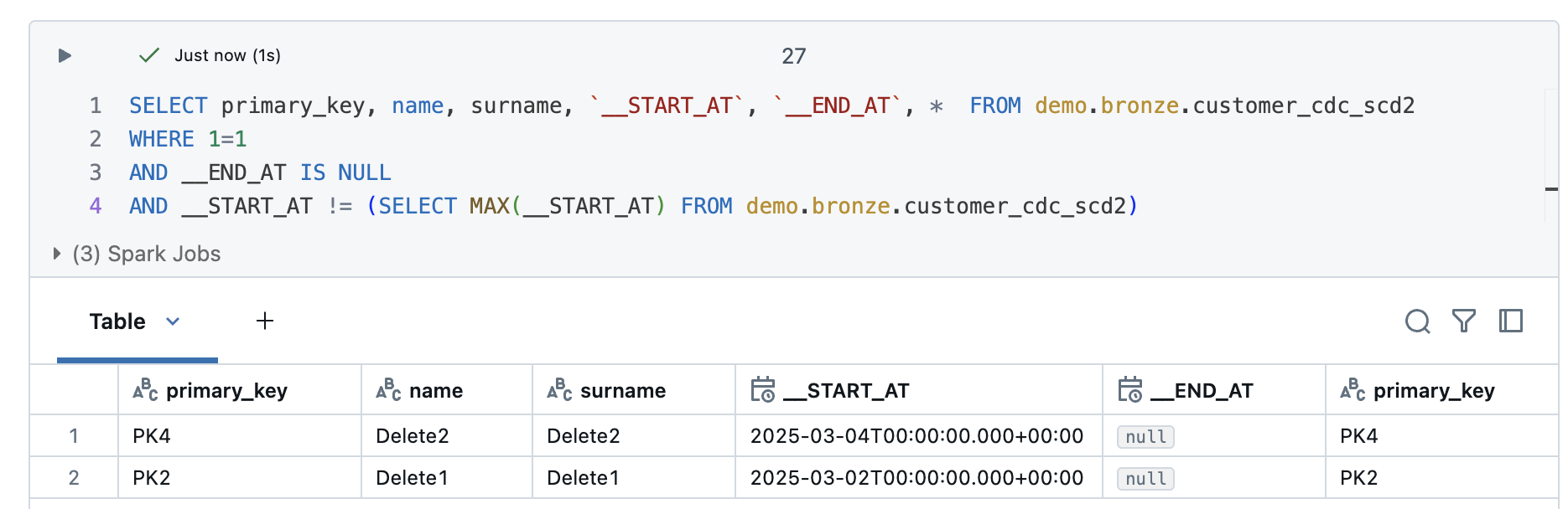
Even with a full reflesh, the deletes are still recognised correctly.

Theoretically, you could now adapt the DLT pipeline and add a second step in which the deleted records are detected with this query and then removed from the bronze table or at least flagged as deletes.

For this purpose, I create a materialised view that reads the data from the SCD2 table and only displays the deleted records. I take the logic from the SQL query.

1
2
3
4
5
6
7
8
9

cdc_scd2_deletes = "cdc_scd2_deletes"

@dlt.table(
  name=cdc_scd2_deletes)

def filter_deletes():
    return dlt.read("demo.bronze.customer_cdc_scd2").alias("c").where(
        "c.__END_AT IS NULL AND c.__START_AT != (SELECT MAX(__START_AT) FROM demo.bronze.customer_cdc_scd2)"
    )

At the same time, I create a view that only contains the active records without deletes.

1
2
3
4
5
6
7
8
9

cdc_view_active = "cdc_scd2_active"

@dlt.table(
  name=cdc_view_active
)
def filter_active():
    return dlt.read("demo.bronze.customer_cdc_scd2").alias("c").where(
        "c.__END_AT IS NULL AND c.__START_AT = (SELECT MAX(__START_AT) FROM demo.bronze.customer_cdc_scd2)"
    )

And why not another view that shows the SCD2 table without deletes but with history. Here the definition is a bit longer, as I first have to find all records with an end date and then those that appear in the deletes.

 1
 2
 3
 4
 5
 6
 7
 8
 9
10
11
12
13
14
15
16
17
18
19
20
21
22
23

cdc_view_final = "cdc_scd2_final"

@dlt.table(
  name=cdc_view_final
)
def filter_active():
    return spark.sql("""
        SELECT * 
        FROM demo.bronze.customer_cdc_scd2 c
        WHERE 
            -- Keep all rows with an end date
            c.__END_AT IS NOT NULL 
            
            -- Keep active rows (__END_AT IS NULL), but only if they are not in the deleted ones
            OR (
                c.__END_AT IS NULL
                AND c.primary_key NOT IN (
                    SELECT primary_key 
                    FROM demo.bronze.cdc_scd2_deletes
                    WHERE __END_AT IS NULL
                )
            )
    """)

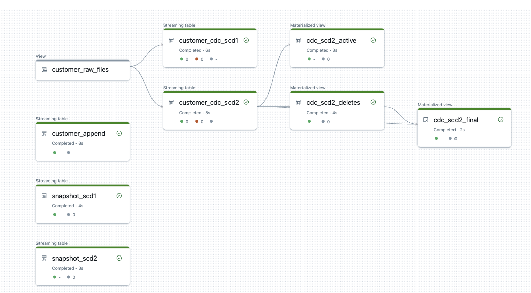
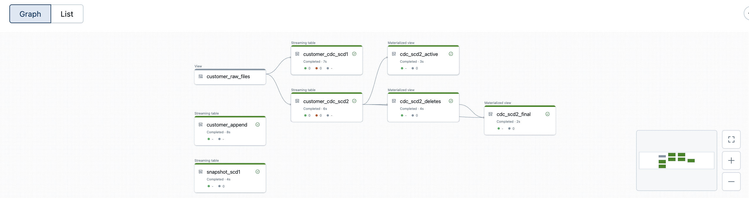
The DLT pipeline now looks like this.

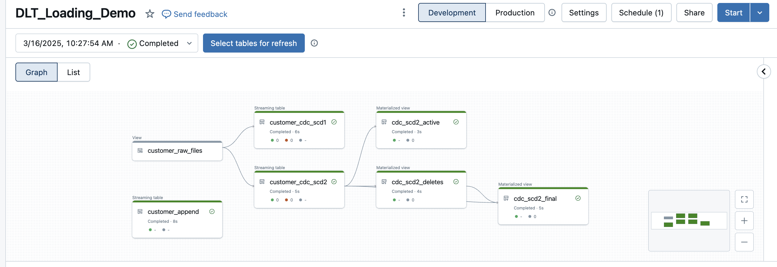
The view with the deletes correctly returns only the deleted records.

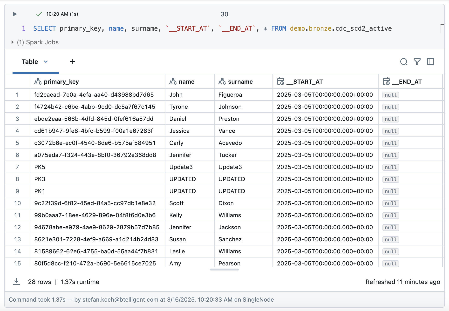
The view with the active records also looks good. I only get those that are actually active.

And lastly, the final view, which should show me both the history, but please filter out the corpses of the deleted ones.

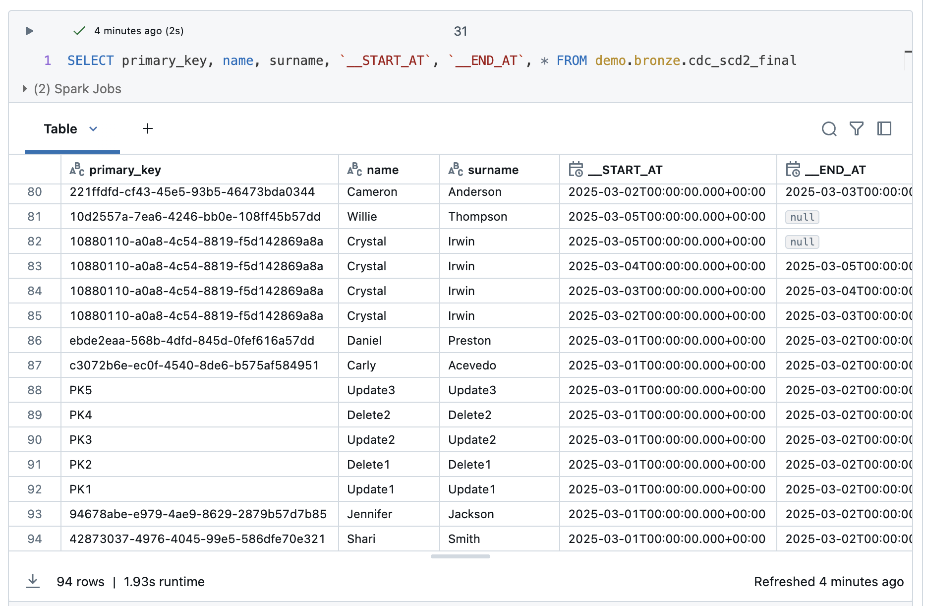
I have 94 rows, which is 2 rows less than in the SCD2 table. These are probably the deletes. I check this with a small query to look at the PK2 and PK4 rows.

Looks good, because we now have the history, but no more corpses with entries without an end time.

But is there an easier solution? Yes, it is possible with the apply_changes_from_snapshot function.

From Change Tracking (CDC SCD2) to Change Tracking Snapshot SCD1

The apply_changes_from_snapshot function is designed precisely for processing snapshots with Delta Live Tables. Here is the documentation: https://docs.databricks.com/aws/en/dlt/python-ref#change-data-capture-from-database-snapshots-with-python-in-dlt

But, unfortunately, I cannot use the Databricks autoloader here. This means that I now have to implement a function that provides me with the exact path of the snapshot file and then another function that provides the next file. In the official documentation, this was realised with an increment if the snapshot file has a version number. I cannot do this as I simply have a snapshot by date. What I can do, however, is to increment the date. In my example setup, I get a new snapshot every day, so I increase the increment by one day.

Again, I start with the version of SCD1. The definition of the DLT looks like this.

 1
 2
 3
 4
 5
 6
 7
 8
 9
10
11
12
13
14
15
16
17
18
19
20
21
22
23
24
25
26
27
28
29
30
31
32
33
34
35
36
37
38
39
40
41
42
43
44
45
46
47
48
49
50

def exist(file_path):
    # Checks if the file exists (location-dependent)
    try:
        dbutils.fs.ls(file_path)
        return True
    except:
        return False

# Function to determine the next snapshot based on date
def next_snapshot_and_version(latest_snapshot_version):
    # If no previous snapshot exists, start with the first day (replace with start date)
    if latest_snapshot_version is None:
        latest_snapshot_date = date(2025, 3, 1)
    else:
        latest_snapshot_date = datetime.strptime(str(latest_snapshot_version), "%Y%m%d") + timedelta(days=1)

    # Create the path to the next snapshot
    next_version = latest_snapshot_date.strftime("%Y%m%d")

    file_path = f"/Volumes/demo/source/raw/customer/Year={latest_snapshot_date.year}/Month={latest_snapshot_date.month}/Day={latest_snapshot_date.day}/"

    if exist(file_path):
        df = spark.read.option("basePath", file_path).parquet(f"{file_path}*").select("*", col('_metadata'))

        # Add the filename by extracting it from _metadata.file_path
        df = df.withColumn("file_name", col("_metadata").getField("file_name"))

        # Extract timestamp using regex
        df = df.withColumn("filename_timestamp_str", regexp_extract("file_name", r"(\d{14})", 1))
        df = df.withColumn("filename_timestamp", to_timestamp("filename_timestamp_str", "yyyyMMddHHmmss"))

        df = df.withColumn("dlt_load_timestamp", (current_timestamp()))
        
        # drop unnecessary columns
        df = df.drop("filename_timestamp_str")
        df = df.drop("file_name")
        
        return df, int(next_version)
    
    else:
        return None

dlt.create_streaming_live_table("snapshot_scd1")

dlt.apply_changes_from_snapshot(
    target="snapshot_scd1",
    source=next_snapshot_and_version,
    keys=["primary_key"],
    stored_as_scd_type=1
)

Firstly, the exist() function is used to check whether a specific directory exists. To do this, dbutils.fs.ls() is used, which returns a list of the directory contents. If the directory does not exist, an exception is caught and False is returned.

To determine the next available snapshot, the date of the last snapshot is used. If no previous snapshot exists, a specified start date is used, otherwise the date of the last snapshot is incremented by one day. This date is then converted into a numerical version number in order to manage the snapshot history. this is hard-coded in my example. This would have to be solved dynamically in a productive pipeline. However, I will not do this in my example.

After the next possible snapshot date has been determined, the system checks whether the corresponding data exists. If so, it is read in as a DataFrame, whereby metadata is loaded in addition to the actual data. The additional metadata is handled in exactly the same way as the other tables.

The customised DLT pipeline now looks like this.

Instead of several steps, this new streaming table can process the data directly. Since we have SCD1, it is a current image of the source table and we do not find any information about the history.

We have exactly the same information as in the source table. Both the content and the number of rows are identical.

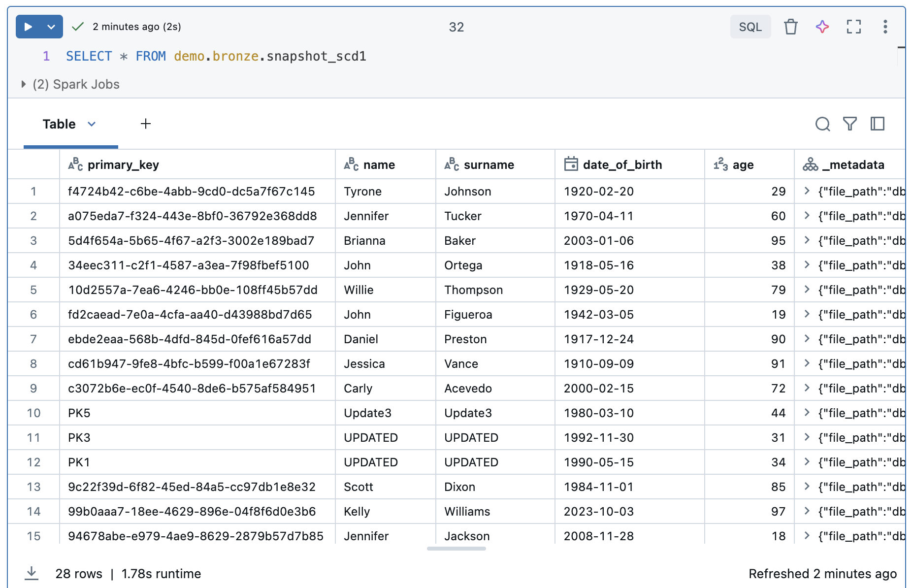
It looks like deletes are also recognised automatically.

Let’s take a look at the SCD2 case when we implement apply_changes_from_snapshot with SCD2.

From Change Tracking Snapshot SCD1 to Change Tracking Snapshot SCD2

The implementation with SCD2 is relatively simple. The logic is almost the same as for SCD1, but we still have to specify which columns we do not want to compare, namely all columns with additional meta information. The last lines are therefore different to SCD1:

1
2
3
4
5
6
7

dlt.apply_changes_from_snapshot(
    target="snapshot_scd2",
    source=next_snapshot_and_version,
    keys=["primary_key"],
    stored_as_scd_type=2,
    track_history_except_column_list = ["_metadata", "filename_timestamp", "dlt_load_timestamp"]
)

The whole code then looks like this:

 1
 2
 3
 4
 5
 6
 7
 8
 9
10
11
12
13
14
15
16
17
18
19
20
21
22
23
24
25
26
27
28
29
30
31
32
33
34
35
36
37
38
39
40
41
42
43
44
45
46
47
48
49
50
51
52

def exist(file_path):
    # Prüft, ob die Datei existiert (Speicherort-abhängig)
    try:
        dbutils.fs.ls(file_path)
        return True
    except:
        return False

# Function to determine the next snapshot based on date
def next_snapshot_and_version(latest_snapshot_version):
    # If no previous snapshot exists, start with the first day (replace with start date)
    if latest_snapshot_version is None:
        latest_snapshot_date = date(2025, 3, 1)
    else:
        latest_snapshot_date = datetime.strptime(str(latest_snapshot_version), "%Y%m%d") + timedelta(days=1)

    # Create the path to the next snapshot
    next_version = latest_snapshot_date.strftime("%Y%m%d")
    
    file_path = f"/Volumes/demo/source/raw/customer/Year={latest_snapshot_date.year}/Month={latest_snapshot_date.month}/Day={latest_snapshot_date.day}/"

    if exist(file_path):
        df = spark.read.option("basePath", file_path).parquet(f"{file_path}*").select("*", col('_metadata'))

        # Add the filename by extracting it from _metadata.file_path
        df = df.withColumn("file_name", col("_metadata").getField("file_name"))

        # Extract timestamp using regex
        df = df.withColumn("filename_timestamp_str", regexp_extract("file_name", r"(\d{14})", 1))
        df = df.withColumn("filename_timestamp", to_timestamp("filename_timestamp_str", "yyyyMMddHHmmss"))

        df = df.withColumn("dlt_load_timestamp", (current_timestamp()))
        
        # drop unnecessary columns
        df = df.drop("filename_timestamp_str")
        df = df.drop("file_name")
        
        return df, int(next_version)
    
    else:
        return None

dlt.create_streaming_live_table("snapshot_scd2")

dlt.apply_changes_from_snapshot(
    target="snapshot_scd2",
    source=next_snapshot_and_version,
    keys=["primary_key"],
    stored_as_scd_type=2,
    track_history_except_column_list = ["_metadata", "filename_timestamp", "dlt_load_timestamp"]
)

And the customised version of the DLT pipeline.

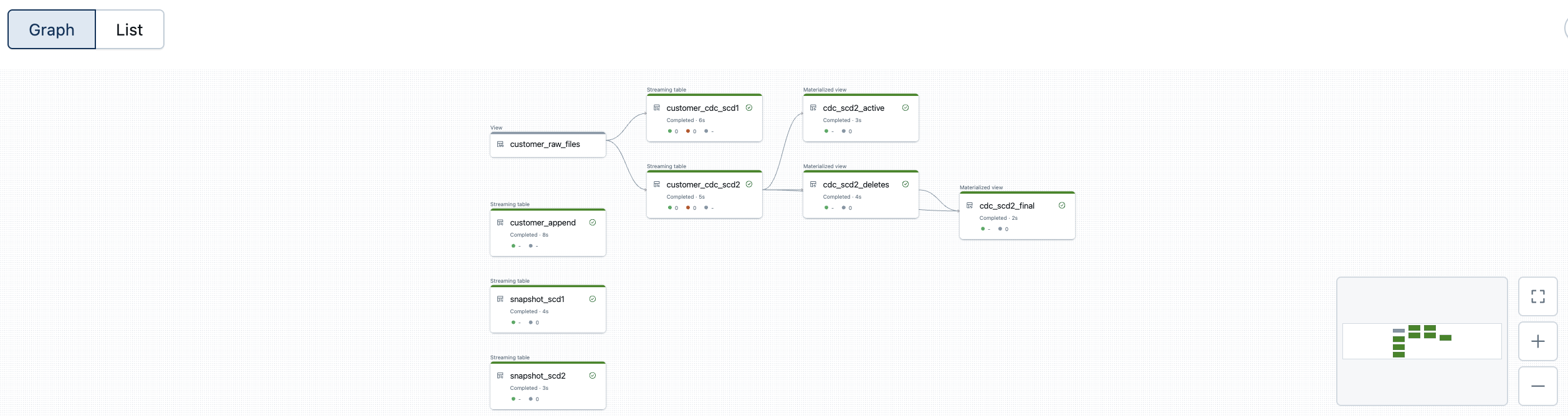
The data looks correspondingly good. The data is fully historicised thanks to the implementation of Slowly Changing Dimension Type 2, which also recognises deleted entries. The function automatically checks whether data records with a specific primary key exist in the target table but no longer appear in the source data record. Such entries are marked as deleted and recorded accordingly in the history.

Conclusion

With the APPLY CHANGES APIs, Delta Live Tables provide a powerful tool with which data from sources with full snapshots can be easily and efficiently integrated into the data platform. There are several approaches that can be followed.

The Append Only method is not recommended because the amount of data explodes here and the data cannot be processed further without further ado.

Latest Record only makes sense if, according to the requirements, no historisation is needed.

Apply Changes SCD1 makes no sense, as you lose the deletes and the historisation. You can go straight back to Latest Record.

The advantage of Apply Changes SCD2 is that you can use Databricks Autoloader. Ingestion is therefore relatively simple. However, additional views must then be installed in order to recognise the deletes.

Apply Changes From Snapshot SCD1: Here too, I doubt that the effort is worth it. You can recognise the deletes, but there is no historisation. You can go straight back to Latest Record.

Apply Changes From Snapshot SCD2: Here I have the complete historisation including delete detection. The ingestion is a bit more complex because you can’t use autoloaders, but the result is a single bronze table.

In conclusion, it can be said that the two methods Apply Changes SCD2 and Apply Changes From Snapshot SCD2 are the most suitable. Depending on how the ingestion is to be suspended, one or the other method is more suitable.

The code for these examples can be found in my public Github repository: https://github.com/stefanko-ch/Databricks_Dojo/tree/main/DLT_Snapshot_Loading

There you can recreate the whole setup 1:1.